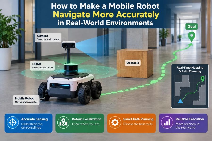

A mobile robot can drive perfectly across a clean lab floor and still lose its way in a busy warehouse, a sunlit hallway, or a cluttered workshop. A wheel slips on dust, a pallet changes position, sunlight washes out a camera image, and a location estimate that was “close enough” suddenly is not.
These failures are not usually caused by one bad sensor or one line of code. Navigation accuracy emerges from a chain of decisions: how the robot moves, what it senses, how it represents the environment, and how it responds when its confidence is low.
For students, this is where textbook localization becomes a real engineering problem. For working engineers, it is where a promising prototype becomes a dependable system that can operate through normal variation rather than only ideal demonstrations.
More accurate navigation does not mean buying every sensor available. It means designing a system whose errors are observable, bounded, and recoverable.
🧭 Define “Accurate” Before Improving Anything
Navigation accuracy has several meanings. A delivery robot may need to arrive within a few centimeters of a charging dock, while an inspection robot may only need to follow the correct corridor and avoid obstacles.
Separate the requirements into position error, heading error, route-following error, obstacle clearance, and task completion. A robot that knows its position but approaches a shelf at the wrong angle may still fail its task.
Also define the operating conditions: floor material, speeds, lighting, people, slopes, expected clutter, and whether a human can intervene. A requirement without conditions is difficult to test honestly.
🗺️ Start With the Right Coordinate Frames
Most navigation problems become easier to diagnose when coordinate frames are explicit. Common frames include map for the fixed environment, odom for locally smooth motion estimates, base_link for the robot body, and sensor frames for cameras or lidar.
Every transform must answer a simple question: where is this measurement, and when was it taken? A small error in a camera-to-robot transform can look like a localization error even when the localization algorithm is working correctly.
Document frame conventions early, including axis directions and units. Mixing millimeters with meters or reversing an axis can produce errors that appear mysterious because the robot still moves plausibly.
🛞 Treat Wheel Odometry as an Estimate, Not Ground Truth
Wheel encoders measure wheel rotation, then infer robot motion from wheel geometry. This process, called odometry, is smooth and fast, but it cannot directly detect a wheel that spun without moving the chassis.
Odometry error accumulates over distance. A differential-drive robot can drift because its wheel diameters differ slightly, its axle width is incorrect in software, or one wheel experiences more traction than the other.
Use odometry for short-term continuity, not as the robot’s final answer about global position. It is the useful “dead reckoning” layer that other sensors must periodically correct.
📏 Calibrate Wheel Geometry on the Actual Robot
Nominal wheel radius and track width are starting values, not calibrated parameters. Tire compression, hub mounting, wear, and payload can all change the effective rolling radius.
Drive straight over a measured distance and compare encoder-derived travel with the real displacement. Then command in-place rotations and compare the measured heading change with the expected angle. Repeat on the surface where the robot will work.
- Correct consistent distance-scale error by adjusting effective wheel radius.
- Correct consistent turning error by adjusting effective track width or wheel-scale imbalance.
- Validate with paths that were not used during calibration, such as a rectangle and a figure eight.
Calibration is not permanent. Recheck it after replacing wheels, changing tire pressure, modifying payload, or moving to a substantially different floor.
🧱 Recognize Slip Before It Becomes Drift
Slip is especially likely during acceleration, sharp turns, braking, ramps, wet surfaces, cable crossings, and transitions between floor types. A robot may appear mechanically stable while its encoder estimate is already diverging.
Compare expected motion with independent evidence. An inertial measurement unit (IMU) may reveal that the body did not rotate as encoder data suggests; scan matching may show that the environment did not move as predicted.
Do not assume every mismatch is sensor noise. Repeated mismatch in particular locations often points to a physical cause: poor traction, a caster that binds, uneven loading, or a controller that commands motion too aggressively.
🎛️ Tune Motion Control Before Blaming Localization
A localization system cannot fully compensate for erratic motion. If wheel-speed control overshoots, oscillates, or gives different responses on each side, the robot’s motion model becomes less trustworthy.
Tune low-level velocity control with safe, repeatable tests. Watch commanded velocity, measured wheel velocity, body rotation, and stopping distance. A stable controller reduces slip and makes sensor fusion assumptions more realistic.
Acceleration and angular-velocity limits matter as much as top speed. Slower, predictable motion can improve total task time when it prevents repeated recovery behavior.
🧠 Use a Motion Model That Matches the Chassis
A navigation filter predicts where the robot should be after a command or odometry update. That prediction depends on a motion model: an approximation of how the chassis actually moves.
Differential drive, Ackermann steering, mecanum wheels, tracked vehicles, and omnidirectional bases do not share the same kinematics. Applying a convenient but inaccurate model creates systematic error that no amount of parameter tuning completely removes.
Include realistic uncertainty. For example, a robot turning quickly on polished concrete should report less confidence in its predicted pose than one moving slowly in a straight line on high-friction flooring.
🌀 Add an IMU for Short-Term Orientation Awareness
An IMU combines accelerometers and gyroscopes. Gyroscopes are particularly useful for measuring short-term angular motion, helping a robot maintain heading when wheel encoders are affected by uneven traction.
However, an IMU is not a magic compass. Gyroscope bias accumulates over time, accelerometers also sense gravity and vibration, and magnetic heading can be distorted by steel shelving, motors, wiring, and building structure.
Mount the IMU rigidly near the chassis when possible. Flexible mounting or vibration can contaminate measurements and make a filter interpret mechanical noise as motion.
⏱️ Synchronize Sensor Time Stamps
A robot moving at speed can travel a meaningful distance while a camera exposure, lidar scan, and encoder message are being processed. If their timestamps are inconsistent, the system combines observations from different moments as though they were simultaneous.
Use source timestamps where available, keep clocks synchronized, and measure transport and processing delay. This is particularly important for cameras, networked sensors, and computers running heavy perception workloads.
A practical clue is an error that grows with speed or angular velocity. If map alignment looks acceptable while stationary but shifts during turns, timing deserves investigation.
📐 Calibrate Sensor Extrinsics Carefully
Extrinsic calibration describes a sensor’s position and orientation relative to the robot body. A lidar mounted a few degrees off-level may produce map mismatches that vary with wall distance. A forward camera whose yaw is wrong can bias visual landmarks sideways.
Measure mounts carefully, but do not rely only on tape-measure values. Validate calibration by viewing known geometry from multiple robot poses. The best calibration is one that improves residual errors across many observations, not merely one convenient scene.
Protect mounts from vibration and accidental bumps. A calibration that was correct on Monday may be wrong after a field repair.
🔦 Choose Sensors for the Environment, Not the Spec Sheet
Each sensing modality has strengths and failure modes. Lidar often provides reliable geometric structure indoors, cameras can recognize rich visual detail, depth cameras provide nearby shape information, and wheel encoders remain inexpensive and fast.
| Sensor or source | Useful contribution | Common limitation |
|---|---|---|
| Wheel encoders | Fast local motion estimate | Slip and accumulated drift |
| IMU | Short-term rotation and dynamics | Bias, vibration, magnetic disturbance |
| 2D or 3D lidar | Geometric localization and obstacle shape | Glass, rain, sparse or repetitive geometry |
| Camera | Visual landmarks and semantic context | Lighting, blur, occlusion, exposure |
| GNSS outdoors | Broad global position reference | Obstruction and reflected signals near structures |
Select sensors by testing difficult conditions, not only nominal ones. A camera-only solution may be excellent in controlled lighting and unsuitable for a loading dock that alternates between darkness and direct sun.
🧩 Fuse Complementary Measurements
Sensor fusion combines sources so that one can compensate for another’s weakness. A typical estimator uses encoders and an IMU for frequent predictions, then uses lidar, vision, GNSS, or known markers to correct gradual drift.
Kalman-filter variants are common when uncertainty and system behavior can be modeled reasonably. Particle-filter localization is also widely used for matching observations to a known map, especially when the initial pose is uncertain.
The key idea is not a particular algorithm name. The estimator should weigh measurements according to their reliability at that moment rather than treating every input as equally trustworthy.
📊 Tune Uncertainty Instead of Forcing Agreement
Filters use covariance, a mathematical description of expected uncertainty. If encoder uncertainty is set unrealistically low, the estimator may cling to a wrong odometry path and reject useful external corrections.
If every sensor is assigned excessive uncertainty, the result can become sluggish and vague. Tuning should reflect observed behavior: repeat tests, log innovations or residuals, and look for measurements that disagree more than the model predicts.
Noise values are not decorative configuration fields. They encode engineering assumptions about traction, vibration, mounting, timing, and environmental conditions.
🏢 Build Maps That Represent Stable Structure
A localization map should emphasize features likely to remain: walls, pillars, permanent machinery, and structural corners. Temporary boxes, parked vehicles, open doors, and movable shelving make poor anchors.
For lidar-based maps, collect scans while moving slowly enough to limit distortion and cover the environment from useful viewpoints. Remove obvious dynamic artifacts if your mapping workflow supports it.
A map is a model, not a photograph. Its job is to help the robot recognize where it is, so stable geometry matters more than visual completeness.
🔁 Plan for Map Change and Version Control
Real facilities change. A remodeled aisle, shifted rack, or newly installed partition can create persistent localization residuals, even though the robot hardware is healthy.
Version maps and record where and when they are valid. Before replacing a map, compare logs from the old and new environments so that a map change does not hide an unrelated sensor fault.
Where change is frequent, consider maps with separate static and dynamic layers. This lets the robot localize against enduring structure while treating routine clutter as obstacles rather than map errors.
🧱 Avoid Repetitive Geometry Traps
Long identical corridors, evenly spaced racks, and blank walls can make several positions look similar to a localization system. The robot may settle on a plausible but incorrect pose, known as an aliasing problem.
Add distinctive information where practical: fiducial markers, unique signs recognized by vision, deliberately placed reflectors, or map regions that include intersecting geometry. These additions are not “cheating”; they are infrastructure for reliable automation.
Route design can help too. A robot that briefly observes a junction or known landmark before entering a repetitive aisle has a stronger starting estimate.
👁️ Make Vision Robust to Real Lighting
Vision localization can fail because of glare, shadows, motion blur, dirty lenses, auto-exposure changes, or seasonal visual changes near windows. These are routine operating conditions, not edge cases.
Use controlled illumination where the environment permits, shield lenses from direct glare, and set exposure strategies appropriate to motion. Evaluate image quality at the robot’s actual speed, not only when it is parked.
Visual features should be paired with geometric or inertial information when reliability matters. A camera can add valuable context, but it should not be asked to ignore physics and lighting.
🌦️ Account for Outdoor and Transitional Zones
Doorways, ramps, courtyards, and loading bays are difficult because several conditions change at once: light, temperature, surface friction, GNSS visibility, and people or vehicles moving through the space.
Model these areas explicitly in testing. A robot may need different speed limits, sensor confidence settings, or obstacle policies near a doorway than in a protected indoor aisle.
For outdoor systems, GNSS can provide a useful global reference, but reflected signals and obstructions near buildings can degrade accuracy. Combine it with local sensing rather than assuming it is uniformly precise.
🚧 Separate Localization From Obstacle Avoidance
A robot needs both a global pose estimate and a current view of nearby hazards. These are related but distinct jobs. A chair should trigger avoidance even if it is absent from the long-term map; it should not necessarily cause the robot to rewrite its map.
Use local costmaps or equivalent short-range representations to capture people, carts, doors, and other dynamic obstacles. Decay or clear these observations appropriately so a moved object does not become a permanent phantom barrier.
Keeping the layers separate makes debugging clearer: is the robot lost, blocked, or simply taking an overly cautious route?
🛤️ Match Path Planning to Robot Footprint
A path that works for a point on a screen may be impossible for a real robot with width, turning radius, sensor overhangs, and braking distance. Inflate obstacles by a safety margin that reflects both physical size and localization uncertainty.
Too little inflation invites clipping shelves and corners. Too much inflation makes usable passages disappear, causing unnecessary detours or apparent planning failures.
Test paths with the full footprint, including loads that extend beyond the base. A robot carrying a bin can have a very different clearance envelope from an empty robot.
🎯 Improve Docking With Local References
Charging and pickup stations usually require more precision than hallway travel. Asking a global map to provide docking-level accuracy can be inefficient, particularly after long runs with small residual uncertainty.
Use a local final-approach method: a fiducial marker, reflective target, short-range lidar geometry, a depth sensor, mechanical guides, or contact-based alignment. The global navigator gets the robot near the station; the local method completes the task.
Mechanical design matters here. Funnel-shaped guides, compliant contacts, and sensible connector placement can make a robust system without demanding unrealistic localization precision.
🧪 Test With Repeatable Ground Truth
You cannot improve accuracy you do not measure. Establish a reference using surveyed landmarks, floor markers, motion-capture equipment where available, or carefully measured test routes. The suitable method depends on required accuracy and workspace size.
Measure more than final error. Record cross-track error, heading error, docking success, recovery frequency, and behavior after deliberate disturbances such as a pushed chassis or a blocked route.
Run the same scenario repeatedly. One successful route may be luck; repeatability reveals whether the system is actually stable.
📁 Log Enough Data to Reproduce Failures
When a robot navigates badly, a video alone rarely explains why. Log raw or near-raw sensor data, timestamps, transforms, wheel commands, estimated pose, covariance, planner decisions, and software version information.
Replayable logs let engineers compare algorithm changes against the same event. They also distinguish a genuine field condition from a regression introduced by a new configuration.
Protect storage and privacy appropriately, especially for camera data in shared workplaces. Useful logging should be intentional, not indiscriminate.
🔍 Diagnose Errors by Their Pattern
Error shape often reveals its source. A gradual position drift during normal travel suggests odometry or estimator issues. Sudden jumps can indicate ambiguous scan matching, visual relocalization errors, or timing problems.
- Error that grows during turns: inspect wheel geometry, IMU alignment, timing, and angular controller behavior.
- Error near metal structures: investigate magnetic interference and lidar reflections or occlusion.
- Error only in sunlight: inspect camera exposure, lens flare, and depth-sensor limitations.
- Error after map updates: compare static features and transform conventions between versions.
Form a testable hypothesis before changing parameters. Random tuning can make one route look better while hiding the underlying cause.
⚠️ Design Clear Recovery Behaviors
No practical localization system is correct all the time. The safer question is what the robot does when confidence drops, observations conflict, or the route becomes blocked.
Recovery may include slowing down, stopping, rotating to acquire more features, returning to a known landmark, requesting assistance, or switching to a constrained safe mode. The response should match the operational risk.
Do not let a robot continue confidently with a poor pose estimate. A conservative pause can be far less disruptive than driving into a restricted area or colliding with equipment.
🛡️ Validate Safety Independently of Navigation Quality
Accurate localization supports safety, but it is not a safety guarantee. People can enter blind spots, sensors can fail, and maps can become stale.
Use independent protective measures appropriate to the platform and environment: emergency stopping, speed limits, protective sensing, physical bumpers, supervised testing, and clear operating boundaries. Applicable safety requirements depend on the machine, jurisdiction, and deployment context, so qualified review is necessary.
Never use a good navigation demo as evidence that all hazards have been addressed.
🧰 Build a Practical Improvement Sequence
Teams often waste time replacing algorithms before establishing basic measurement quality. A more effective sequence is to improve the cheapest, most observable causes first.
- Verify frames, units, timestamps, and sensor mounting.
- Calibrate wheel geometry and stabilize low-level motion control.
- Collect logs and define repeatable accuracy tests.
- Improve maps and sensor coverage in failure locations.
- Tune fusion uncertainty using measured residuals.
- Add local references or infrastructure where the task needs high precision.
- Validate recovery and safety behavior under realistic disturbances.
This order does not fit every robot, but it reduces the chance of using complex software to conceal a basic mechanical or integration fault.
🤝 Design the Environment When You Can
Robot navigation is a system property, not only a robot property. Better lighting, cleaner sightlines, stable storage rules, protected charging zones, and thoughtfully placed landmarks can improve reliability more than a marginal sensor upgrade.
This does not mean environments must be rebuilt around machines. It means recognizing that small operational changes can reduce uncertainty at the places where precision matters most.
In a warehouse, for example, keeping a docking approach clear and adding a durable local marker may be more effective than demanding centimeter-level global localization throughout every aisle.
📈 Maintain Accuracy After Deployment
Navigation performance changes over time as wheels wear, lenses collect dust, mounts loosen, maps age, and facility routines evolve. Include periodic calibration checks and scenario-based regression tests in maintenance planning.
Monitor leading signals, such as rising localization residuals, increasing recovery events, or longer docking times. These trends can reveal degradation before it becomes a visible operational failure.
When changes are made, alter one well-documented factor at a time when feasible. This preserves the ability to explain whether the change helped.
🧭 The Core Principle: Manage Uncertainty End to End
Accurate mobile robot navigation is not achieved by declaring one sensor “best.” It comes from combining calibrated mechanics, suitable sensors, correctly timed data, realistic uncertainty models, stable maps, task-specific local guidance, and deliberate recovery behavior.
The most capable systems know when they are uncertain. They slow down, seek better observations, use redundancy, and avoid pretending that an estimate is more precise than the evidence supports.
A robot navigates more accurately in the real world when its entire system is designed to detect, limit, correct, and safely recover from error. Build that discipline into hardware, software, environment design, and testing, and accuracy becomes a repeatable engineering outcome rather than a lucky demonstration. 🦾🧭