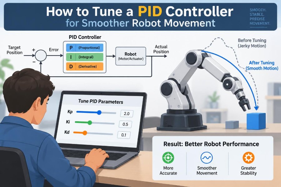

A mobile robot reaches a waypoint, overshoots it, corrects too hard, and begins to wobble from side to side. A robotic arm stops near its target but leaves a small, persistent position error. A drone holds altitude well indoors, then reacts poorly when its battery voltage falls.
These situations often look like mechanical problems, but the control loop is frequently part of the story. A PID controller can turn a noisy, hesitant machine into one that moves predictably—or make an otherwise sound robot oscillate, heat its motors, and miss its marks.
Tuning PID gains is not about discovering three magic numbers. It is a disciplined process of defining the behavior you need, measuring what the robot actually does, changing one factor at a time, and respecting physical limits.
This guide focuses on practical tuning for real robot motion: wheels, arms, linear axes, and other systems where smooth tracking matters as much as reaching the final position.
🎯 Start with the motion you actually need
“Smooth” is not a single measurable requirement. A warehouse robot may need low overshoot to avoid shelves, while a line-following robot may accept a little overshoot in exchange for tighter path tracking. An arm carrying liquid may prioritize gentle acceleration over raw speed.
Define the task before changing gains. Useful criteria include settling time, maximum overshoot, steady-state error, vibration, current draw, and repeatability. A controller cannot optimize every criterion equally well, so identify the ones that matter most.
🔁 Understand the closed loop
A closed-loop controller repeatedly compares a setpoint—the desired position, speed, angle, or temperature—with a measured value from a sensor. The difference is the error. PID uses that error to calculate a command for the motor driver or actuator.
The loop runs many times per second. The actuator changes the robot, the sensor reports the new state, and the controller reacts again. Delay, sensor noise, friction, actuator limits, and software timing all influence this cycle.
➕ What proportional control contributes
The proportional term applies an output related to the current error: P = Kp × error. A larger position error produces a stronger correction. If a wheel is far below its requested speed, proportional control asks for more motor effort.
Increasing Kp usually makes a robot react more quickly and feel less sluggish. But too much proportional gain creates overshoot and oscillation because the robot’s momentum carries it beyond the target while the controller is still commanding a strong correction.
🧮 What integral control corrects
The integral term accumulates error over time: I = Ki × ∫error dt. It addresses errors that remain even after proportional control has done most of its work. These errors often come from static friction, gravity, a biased sensor, or a load that continuously resists motion.
For example, an arm joint may need a small continuing torque to hold position against gravity. Proportional control alone may settle with a slight droop; integral action gradually adds enough output to remove it.
⚡ What derivative control predicts
The derivative term responds to how rapidly error changes: D = Kd × de/dt. It acts like damping. When a robot approaches its target quickly, derivative action can reduce the command before momentum carries the mechanism too far.
Derivative control is especially useful for position loops with flexible or moving loads. Its weakness is noise: differentiating a noisy encoder or IMU signal can create a jittery output. Filtering and careful implementation matter as much as the value of Kd.
🧠 Read the full PID equation carefully
A common discrete-time implementation is u[k] = Kp e[k] + Ki Σe[k]Δt + Kd(e[k] - e[k-1])/Δt. Here, Δt is the actual loop interval. The output u may be motor voltage, PWM duty command, torque command, or a speed request to a lower-level drive.
Different libraries define gains differently. Some fold the sample time into Ki and Kd; others do not. Never copy gains from a tutorial until you understand its controller form, units, output range, and update period.
🧱 Fix mechanical faults before tuning
A PID controller cannot compensate cleanly for a loose coupling, binding gearbox, slipping belt, bent shaft, or intermittent encoder. It may hide the symptom briefly by commanding more effort, but the result is usually noisy motion and fragile tuning.
- Check that the mechanism moves freely through its working range.
- Verify encoder mounting, counts, direction, and electrical connections.
- Inspect backlash, gear wear, belt tension, and structural flex.
- Confirm the motor and driver can supply the required continuous and peak effort safely.
Mechanical repeatability makes tuning repeatable. Without it, gains that work on one run may fail on the next.
📏 Verify sensor scaling and sign conventions
A controller needs measurements in meaningful units. Position might be radians, degrees, millimeters, or encoder counts; velocity might be radians per second or wheel revolutions per minute. Convert consistently and document the choice.
Also test the sign. A small positive command must move the measured state in the positive direction. If the loop runs away immediately, stop it and correct the sign convention. No amount of gain adjustment can repair positive feedback.
⏱️ Keep the control period predictable
PID gains depend on timing. If a nominal 10 ms loop sometimes runs at 10 ms and sometimes at 40 ms because logging or other tasks block it, integral accumulation and derivative estimates become inconsistent.
Use a timer, real-time scheduler, or a dedicated periodic task where possible. Measure the actual interval and pass it to the controller if the implementation supports variable Δt. Run debugging prints and high-volume telemetry outside the time-critical loop.
🛑 Set safe output limits first
Before tuning, clamp the controller output to a safe range for the motor driver and mechanism. Position limits, emergency stops, current limits, and software travel limits should be active when a robot can cause damage or injury.
Begin with low-speed tests, no unexpected payload, and a clear area around the moving parts. A gain trial should reveal behavior, not become a test of whether someone can reach the power switch quickly.
📊 Log the signals that explain behavior
Human observation catches large oscillations but misses timing details. Log the setpoint, measured position or velocity, error, controller output, and each P, I, and D contribution when possible. Motor current and supply voltage are also valuable diagnostics.
Plot these signals against time. A graph can reveal whether a delay comes from the controller, a saturated motor command, a sensor update rate, or a mechanical resonance. Consistent plots are more informative than isolated impressions.
🧪 Choose a repeatable test maneuver
A step test is a practical starting point: command a fixed change in position or speed and record the response. Use the same step size, payload, battery condition, surface, and test path for each comparison.
Also test maneuvers that resemble the real job. A wheel controller tuned only for a no-load speed step may behave differently during turns. An arm joint tuned in one orientation may need different support against gravity in another.
🔇 Begin with integral and derivative disabled
For a first manual tune, set Ki = 0 and Kd = 0. This exposes the basic relationship between proportional gain and the plant—the motor, gearbox, load, and structure being controlled.
Start with a low Kp and apply the chosen test. Increase it gradually until the response becomes prompt but is not persistently oscillatory. Record every trial; otherwise it is easy to lose track of which change caused an improvement.
📈 Raise proportional gain to the useful edge
With too little Kp, the robot moves slowly, lags the command, and may stop well short of target under load. As Kp rises, response becomes faster and steady error often decreases.
Stop increasing when you see sustained oscillation, repeated overshoot, harsh reversals, or audible buzzing. Then reduce Kp modestly. The goal is not the highest possible gain; it is enough authority without exciting unstable or uncomfortable behavior.
🪶 Add derivative damping cautiously
Once proportional control is responsive, add a small Kd if the system overshoots or rings. Increase it in small increments and compare plots. Proper derivative action often shortens the tail of a response and reduces repeated corrections around the target.
If output becomes visibly noisy, especially while the mechanism is still, derivative gain may be too high or the measurement may be too noisy. Reducing Kd, filtering velocity, or calculating derivative from measurement rather than error can help.
🧲 Add integral only for remaining bias
After P and D are satisfactory, introduce a small Ki when a repeatable steady-state error remains. Let the robot settle long enough to show whether the error disappears gradually without creating a slow oscillation.
Integral action is often the last term to add because it has memory. A controller can appear stable for a few seconds, then begin hunting as stored integral correction becomes excessive. Patience during tests prevents false confidence.
🌪️ Recognize the signatures of poor tuning
| Observed behavior | Likely contributors | Useful next check |
|---|---|---|
| Slow, weak response | Kp too low; limited actuator | Check output saturation and raise Kp carefully |
| Fast repeated oscillation | Kp too high; structural resonance | Lower Kp; inspect mechanics and sampling |
| Slow wandering around target | Ki too high | Reduce Ki and inspect integral state |
| Jitter at rest | Kd noise; encoder quantization | Reduce/filter derivative path |
| Persistent offset under load | Too little Ki or feedforward | Add small Ki or model known load |
These are clues, not universal diagnoses. A saturated motor, delayed sensor, or loose mechanism can imitate a gain problem, so use recorded signals to confirm the cause.
🧯 Prevent integral windup
Integral windup occurs when the controller keeps accumulating error while its output is already limited. Imagine commanding an arm beyond a physical stop: the motor cannot move farther, but the integral term continues growing. When the command reverses, the stored correction can cause a large, delayed lunge.
Common protections include clamping the integral state, integrating only when output is not saturated, or using back-calculation to unwind the integrator. Reset or appropriately manage integral state when switching modes, disabling the actuator, or making a large setpoint change.
🚦 Distinguish saturation from bad gains
If the controller output sits at its maximum for much of a move, gain changes may not alter acceleration at all. The system is actuator-limited. Raising Kp further can merely increase overshoot once the robot nears the target.
Check the motor driver’s voltage, current limit, thermal state, battery sag, and gearing. A controller cannot create torque the hardware cannot provide. This distinction is crucial when a robot performs well unloaded but struggles with a real payload.
🛞 Tune velocity loops before position loops
Many robot systems use cascaded control. An inner velocity loop makes motor speed follow a requested speed; an outer position loop generates that speed request. This structure lets the fast inner loop handle motor dynamics while the outer loop handles geometry and motion goals.
Tune the inner velocity loop first, with a realistic load. Then tune the outer position loop more gently. Trying to tune both at once makes it difficult to tell whether poor position tracking comes from the motor-speed loop or the position logic.
🧭 Use feedforward for predictable effort
Feedback reacts after an error appears. Feedforward supplies an expected command in advance, based on what the robot is asked to do. A drive wheel may need a voltage related to requested speed; an arm may need gravity compensation based on joint angle.
Feedforward does not replace PID. It reduces how much correction PID must supply, which can improve tracking without relying on aggressive gains. It needs a reasonably accurate model, so retain feedback for friction changes, disturbances, and model error.
🗺️ Shape setpoints instead of demanding impossible jumps
A step command asks for an instantaneous change that a physical robot cannot produce. The controller responds aggressively because the error is initially large. For smooth movement, generate a trajectory with bounded velocity and acceleration; for sensitive mechanisms, also limit jerk, the rate of acceleration change.
A trapezoidal velocity profile accelerates, cruises, and decelerates. An S-curve softens transitions further. Motion profiling often removes harsh behavior more effectively than reducing PID gains until the robot becomes sluggish.
📡 Treat noisy sensors as a control-design issue
Encoders with low resolution can make low-speed velocity estimates jump between values. IMUs can carry vibration. Potentiometers can add electrical noise. If the controller reacts to these fluctuations, motors chatter and gears experience unnecessary reversals.
Filter measurements only as much as needed. A low-pass filter can reduce noise, but every filter adds delay, and excessive delay can destabilize a fast loop. Improve sensor mounting, shielding, resolution, or estimation before using heavy filtering as a cure-all.
🪛 Account for friction, backlash, and deadband
Static friction means a mechanism may need more effort to begin moving than to keep moving. Backlash means an actuator can reverse before the load responds. Motor-driver deadband means small commands produce no motion. These nonlinear effects are common in practical robots.
A high integral gain may force motion through friction, but it can cause overshoot after the joint breaks free. Better options can include friction compensation, a small controlled minimum command, tighter mechanics, or a trajectory that avoids constant tiny reversals.
🔋 Retest under changing operating conditions
Gains tuned with a fresh battery, cool motors, and no payload are not automatically valid elsewhere. Battery voltage affects available motor speed and torque. Temperature changes winding resistance and friction. Payload changes inertia, and floor material changes wheel traction.
Validate across the operating envelope: expected loads, low and high battery conditions, likely speeds, different directions, and representative temperatures. If one fixed gain set cannot meet the requirements, gain scheduling or improved feedforward may be appropriate.
🦿 Watch for flexible structures and resonance
A long arm, compliant wheel mount, belt drive, or lightweight frame can store and release energy. What appears to be PID oscillation may be a mechanical resonance excited by rapid commands or high gain.
Lower gains may avoid the resonance, but that can sacrifice performance. Structural stiffening, changed gear ratios, altered motion profiles, notch filtering, or moving the control bandwidth away from the resonant frequency can be more durable solutions. These changes require careful testing because filters also affect phase and stability.
🧑💻 Make tuning experiments reproducible
Maintain a tuning record with firmware version, controller equation, gains, loop period, output limits, sensor scaling, test setup, payload, and observed result. Save plots with meaningful names rather than relying on memory.
For team projects, this record prevents a common failure: one person changes a gain, another changes encoder scaling, and the group cannot explain why behavior shifted. Reproducibility turns tuning from trial-and-error into engineering evidence.
🔄 Change one meaningful variable at a time
It is tempting to change all three gains after an unsatisfactory test. That may produce a better-looking response, but it hides causation. Change one gain or one clearly defined design choice, rerun the same maneuver, and compare the result.
There are exceptions: correcting a sign error, replacing a bad sensor, or adding anti-windup can require broader changes. Even then, establish a new baseline before further gain adjustments.
🏭 Consider automated tuning with healthy skepticism
Auto-tuners can estimate useful starting gains by applying controlled tests and identifying aspects of the plant response. They can save time, especially during commissioning, but their result depends on assumptions about noise, delay, linearity, load, and test safety.
Use automated results as candidates, not unquestioned answers. Review output limits, validate real trajectories, and test disturbances. A gain set optimized for a single step response may be unsuitable for a robot that spends its day following curved paths.
⚠️ Avoid common tuning shortcuts
- Copying gains: hardware, units, loop rate, and load differ even between similar robots.
- Tuning only at no load: the real payload may expose saturation and inertia problems.
- Using integral to fix everything: it can mask inadequate mechanics or actuator capacity.
- Filtering blindly: a smooth plot can conceal damaging delay.
- Ignoring output clipping: saturation changes the effective behavior of the loop.
Each shortcut skips information the controller needs to behave predictably in the real system.
✅ Use a practical final validation checklist
Before declaring the controller ready, test both nominal behavior and the awkward cases it will encounter. Confirm that the robot starts, stops, reverses, and recovers from a small disturbance without unexpected oscillation.
- Check position and velocity limits at software and hardware boundaries.
- Review motor temperature and current during representative duty cycles.
- Test sensor dropouts or invalid readings with a safe fallback behavior.
- Verify mode transitions do not release stored integral action.
- Repeat tests after power cycling and with the production configuration.
🧩 The core principle: tune the whole motion system
Smoother robot movement comes from more than P, I, and D values. It comes from a trustworthy sensor, adequate actuator authority, predictable timing, suitable mechanics, a feasible motion profile, and a controller that handles limits gracefully.
A reliable sequence is simple: make the system safe and measurable, verify mechanics and signs, tune proportional response, add damping when needed, add only enough integral to remove persistent bias, then validate across real operating conditions. PID works best when treated as one part of a complete motion-control design.
The best PID tune is the one that meets the robot’s real task smoothly, safely, and repeatably—not the one with the largest gains or the fastest-looking graph. Careful measurement and incremental changes will get you there. 🦾📈🔧