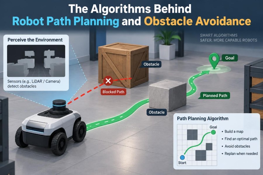

A warehouse robot carrying a tote reaches an aisle blocked by a pallet. A delivery rover encounters a pedestrian stepping off a curb. A robotic arm moves toward a part while a technician’s hand enters its workspace. In each case, the machine must do more than stop: it must decide what space is safe, what route remains useful, and how to move without creating a new problem.
That decision happens through path planning and obstacle avoidance. These related capabilities turn a robot’s sensors, maps, and motion limits into actions. They are central to mobile robots, autonomous vehicles, drones, surgical systems, and industrial manipulators.
The challenge is easy to underestimate. A route that looks clear on a screen may be impossible for a real robot to turn through, unsafe once uncertainty is considered, or obsolete a second later because the environment changed.
Good robot navigation is therefore not one magic algorithm. It is a layered engineering problem: represent the world, search for feasible motion, react to change, and continually verify that the robot can stop or steer safely.
🧭 What Path Planning Actually Means
Path planning is the process of finding a collision-free route from a start configuration to a goal configuration. A configuration describes every variable needed to locate a robot: for a ground robot, that may include x position, y position, and heading; for an arm, it includes its joint angles.
A path is geometric: it says where the robot should go. A trajectory adds time, velocity, acceleration, and sometimes force. This distinction matters because a path can avoid a wall yet still demand an impossible turn or unsafe braking maneuver.
🚧 Why Obstacle Avoidance Is a Different Job
Obstacle avoidance is the short-horizon process of preventing a collision with objects detected now. It is often reactive, operating from sensor observations rather than a complete world model.
A planner might choose the far side of a building as part of a long route. Avoidance handles the cart, person, or opening door that was not in the map. Real systems commonly need both: planning supplies direction, while avoidance protects the robot between planning updates.
🗺️ Start with a Usable World Model
Algorithms can only plan through the world representation they receive. A map may be a floor plan, a 3D point cloud, a set of labeled objects, or a simple grid of occupied and free cells.
For mobile robots, an occupancy grid is common. It divides space into small cells and assigns each a belief about whether it is occupied. Grid resolution is a trade-off: tiny cells preserve detail but increase memory and search time; large cells are efficient but can erase narrow passages.
📍 Localization Comes Before Navigation
To follow any planned route, a robot needs an estimate of its own pose: position and orientation. Wheel encoders, inertial sensors, cameras, lidar, GPS where available, and map matching can all contribute.
Localization is never perfect. Wheel slip, repeated visual textures, sensor noise, and an outdated map can shift the estimated pose. A route with only millimeters of clearance is risky if the position estimate itself may be wrong by more than that.
📐 Configuration Space Makes Robot Size Visible
A useful planning idea is configuration space, often shortened to C-space. Rather than treating the robot as a point moving among obstacles, the planner represents each possible robot configuration as a point in an abstract space.
One practical consequence is obstacle inflation. For a circular mobile robot, obstacles can be enlarged by the robot radius plus a safety margin. Then the robot’s center can be planned as a point. For a robotic arm, C-space has one dimension per joint, which makes the geometry much more complex.
🧱 Safety Margins Are Not Wasted Space
Inflating obstacles accounts for robot dimensions, tracking error, localization uncertainty, and sensor imperfections. The appropriate margin depends on the application: a slow indoor robot with accurate lidar may use less clearance than a fast outdoor platform on uneven ground.
Too little margin causes near-misses and fragile behavior. Too much margin can falsely close corridors and make a workspace appear unreachable. Engineers should choose margins from measured uncertainty and stopping behavior, not visual intuition alone.
🎯 Defining the Goal and the Cost
“Reach the goal” is rarely enough. The planner needs a cost function to compare feasible choices. Distance is useful, but it is only one possible cost.
- Travel time matters for production and delivery tasks.
- Energy matters for battery-powered robots and drones.
- Clearance matters around people, fragile stock, and uncertain obstacles.
- Smoothness matters because sharp turns increase tracking difficulty.
- Risk can penalize areas with poor sensing or changing traffic.
Weights in a cost function express operational priorities. They should be tuned and validated against real behavior, because an elegant mathematical objective can produce undesirable routes if it misses a meaningful constraint.
🔎 Graph Search Turns Maps into Choices
Many planners convert free space into a graph. Nodes represent candidate positions or states, and edges represent allowed moves between them. Planning then becomes a search for a low-cost chain of edges.
This model works naturally with grids, roadmaps, and lattice-based motion primitives. Its strength is clarity: engineers can inspect the states, connections, costs, and rejected transitions when debugging a route.
📏 Dijkstra’s Algorithm Finds Reliable Shortest Paths
Dijkstra’s algorithm expands outward from the start, always finalizing the currently least-cost unexplored node. With nonnegative edge costs, it finds an optimal path through the graph.
Its drawback is that it does not know which direction the goal lies. On a large uniform grid, it may explore a broad area that has little relevance to the destination. It remains valuable when a system needs costs to many locations or when no trustworthy directional estimate is available.
⭐ A* Search Uses a Helpful Estimate
A* improves directed search by adding a heuristic: an estimate of the remaining cost to the goal. On a flat grid, straight-line or Manhattan distance can serve as the estimate, depending on allowed moves.
When the heuristic does not overestimate the true remaining cost, A* can retain optimality while exploring far fewer nodes than Dijkstra’s algorithm. A poor heuristic, however, can offer little speed benefit; an overly optimistic or inconsistent implementation can also complicate guarantees.
🧮 Heuristics Must Match the Robot
A simple straight-line heuristic assumes the robot can move directly in any direction. That is not true for a car-like robot that cannot slide sideways, or for a drone that has climb-rate and turn limits.
More informed heuristics can incorporate kinematic constraints, precomputed motion costs, or distance fields. Better guidance can greatly reduce search, but it must remain computationally worthwhile and compatible with the planner’s assumptions.
🔄 D* and Incremental Replanning
Static-map search becomes inefficient when new obstacles appear repeatedly. Incremental methods such as D* and related approaches reuse information from earlier searches rather than discarding all prior work.
Imagine a warehouse map that is mostly known, while aisles occasionally close. An incremental planner can update affected regions and repair the route. This is especially useful when a robot revisits the same space, although changing sensor data still needs careful filtering to avoid constant route churn.
🌳 Sampling-Based Planning Handles Complex Spaces
Grid search becomes difficult as the number of configuration variables grows. A six-joint arm, for example, has a six-dimensional joint space. Sampling-based planners explore by randomly or strategically selecting valid configurations.
They do not require every possible state to be discretized in advance. This makes them practical for high-dimensional problems, irregular workspaces, and systems with complicated collision geometry.
🌲 Rapidly Exploring Random Trees
A Rapidly Exploring Random Tree, or RRT, grows a tree from the start. It samples a configuration, finds the nearest existing tree node, and extends toward that sample by a limited step if the motion is collision-free.
RRT tends to spread into unexplored regions quickly, which helps with large spaces. Basic RRT does not usually produce a polished route; its paths can be jagged and may require shortcutting, smoothing, or trajectory optimization afterward.
✨ RRT* Trades Speed for Better Paths
RRT* adds rewiring: when a new sample offers a cheaper connection to nearby tree nodes, it can improve their parent relationships. Given continued sampling under suitable assumptions, RRT* approaches an optimal solution.
That theoretical improvement has a practical cost. RRT* typically needs more collision checks and computation than basic RRT. It is often chosen when path quality matters and planning time is available, rather than for every fast reaction cycle.
🕸️ PRM Reuses Routes in Repeated Workspaces
A Probabilistic Roadmap, or PRM, samples many collision-free configurations and connects nearby compatible ones. The resulting graph can answer multiple start-to-goal queries in the same workspace.
PRM is a natural fit for a robot arm that repeatedly works around fixed fixtures. Its weakness is environmental change: if people, carts, or fixtures move often, parts of the roadmap may become invalid and require checking or rebuilding.
🚗 Kinematic Constraints Change the Plan
Geometry alone is not motion. A differential-drive robot can rotate in place, while an automobile-like vehicle has a minimum turning radius. A fixed-wing drone must keep moving forward and cannot make arbitrary tight turns.
Planners that account for these kinematic constraints search over feasible motion segments, not merely neighboring map cells. Common approaches include state lattices and analytically derived curves for car-like motion. Ignoring kinematics is a common reason a route looks correct but cannot be executed.
⚙️ Dynamics and Stopping Distance Add Reality
Dynamics include mass, acceleration limits, tire or wheel traction, actuator capability, and momentum. A robot moving quickly cannot instantaneously turn or stop at an obstacle boundary.
For safety-critical navigation, planning should consider a reachable set of future states and ensure there is a braking or evasive option. A local controller may reduce speed near blind corners because lower speed shortens the distance needed to respond to a new detection.
👀 Sensors Provide Evidence, Not Perfect Truth
Lidar measures ranges well in many settings, cameras provide rich semantic information, radar can be useful in adverse visual conditions, and ultrasonic sensors are inexpensive for close detection. Each has blind spots and failure modes.
Reflective, transparent, dark, distant, or occluded objects can challenge particular sensors. Sensor fusion can improve coverage, but combining inputs does not eliminate uncertainty. A navigation stack should explicitly handle stale data, limited field of view, and confidence rather than treating every observation as exact.
📊 From Measurements to Costmaps
Local navigation often uses a costmap: a nearby grid where obstacles carry high cost and nearby areas carry gradually increasing cost. The gradient encourages the robot to keep clearance rather than scrape past every object at the minimum legal distance.
Costmaps usually combine static map information with current sensor readings. They also need decay rules. If temporary obstacles never clear, the robot may believe an aisle is permanently blocked; if they clear too quickly, it may drive toward an object that is only briefly occluded.
🏃 Local Planners Choose the Next Safe Motion
A global path is an intention, not a motor command. The local planner selects a short feasible movement based on current obstacles, robot velocity, and the nearby portion of the global route.
Methods differ in detail, but their role is similar: evaluate candidate velocities or trajectories, reject collisions, and score the rest by progress, clearance, smoothness, and adherence to the route. The local horizon must be long enough to anticipate stopping needs, not just the next few centimeters.
🌊 Potential Fields Offer Intuitive Guidance
Potential-field methods model the goal as attractive and obstacles as repulsive. Adding those virtual forces yields a direction of motion. The idea is simple and can be effective for smooth, reactive guidance.
Its classic weakness is a local minimum: forces can cancel before the robot reaches the goal, such as in a U-shaped obstacle arrangement. Oscillation in narrow corridors is another risk. Potential fields work best when paired with higher-level planning or escape strategies.
🧠 Model Predictive Control Looks Ahead
Model Predictive Control (MPC) repeatedly predicts robot behavior over a short future horizon, optimizes control inputs, applies the first action, and solves again after receiving new observations.
MPC can incorporate steering limits, speed limits, obstacle clearance, and route-following objectives in one optimization problem. Its trade-off is computational demand and sensitivity to model quality. A solver that cannot reliably meet its timing deadline is unsuitable for real-time control, however attractive its predicted trajectory looks.
🚶 Dynamic Obstacles Need Prediction and Caution
A moving person or forklift is not just an obstacle at its current location. The relevant question is where its possible future motion overlaps the robot’s future motion. Prediction may use measured velocity, traffic rules, or learned behavior models.
Predictions are uncertain, especially around people. Robust behavior often means maintaining extra space, reducing speed, and yielding when intent is ambiguous. Designing for polite, legible motion can be as valuable as minimizing seconds from a route.
🧩 The Global-Local Architecture
Many deployed systems use a hierarchy. A global planner finds a route across the known map. A local planner follows it while avoiding immediate hazards. A controller converts the selected local trajectory into wheel, steering, or joint commands.
This separation makes updates manageable: a new distant blockage can trigger global replanning, while a person crossing nearby is handled locally. The interfaces matter. If the global route assumes a clearance the local layer cannot maintain, or if both layers fight over priorities, the robot can behave indecisively.
🔁 Replanning Is Necessary but Can Become a Problem
Frequent replanning adapts to change, but blindly replacing the route on every sensor fluctuation can create jitter, oscillation, and wasted computation. A robot may repeatedly choose opposite sides of an obstacle without committing to either.
Useful stabilizers include hysteresis, route-change penalties, short-term obstacle tracking, and a minimum progress requirement before reversing a decision. Replanning should be triggered by meaningful changes: blocked progress, invalidated path segments, or a substantially better route.
⚠️ Common Failure Modes in Tight Spaces
Robots frequently fail at the boundary between ideal maps and physical environments. Narrow doorways, glass panels, low overhangs, wheel slip, and objects extending beyond their mapped footprint all expose assumptions.
- Corner cutting: a smoothed path clips inflated obstacles or exceeds turning limits.
- Deadlock: the robot and another agent both wait or repeatedly yield.
- Oscillation: local avoidance alternates left and right without progress.
- False free space: a sensor misses an obstacle because of angle, occlusion, or material.
- Goal trapping: the final pose is geometrically near but dynamically unreachable.
Logging maps, poses, sensor frames, planner decisions, and controller commands is essential for diagnosing which assumption failed.
🧪 Simulation Helps, but Hardware Has the Last Word
Simulation is excellent for testing thousands of layouts, tuning costs, and reproducing rare planner failures. It can model geometry and approximate sensors without risking equipment or people.
But simulations often simplify friction, latency, actuator backlash, sensor artifacts, and human behavior. A sound workflow moves from simulation to controlled physical tests, beginning at low speed and with conservative safety boundaries. Field validation should test the uncomfortable cases, not only clean demonstrations.
🛡️ Safety Is an Architecture, Not a Planner Setting
No ordinary route planner should be the only barrier against harm. Safety functions can include emergency stops, speed limiting, protective zones, independent proximity sensing, fault detection, and defined fallback states.
The exact measures depend on robot type, environment, applicable requirements, and risk assessment. What matters conceptually is independence: if localization degrades or the planning process fails, the system should still have a predictable way to reduce risk rather than continuing on the last command.
🔧 A Practical Algorithm Selection Guide
There is no universal winner. Select methods by workspace structure, robot constraints, timing budget, map quality, and consequence of failure.
| Situation | Often suitable starting point | Key caution |
|---|---|---|
| Known indoor floor map | A* or incremental graph search plus local avoidance | Account for footprint and blocked aisles |
| High-dimensional robot arm | PRM, RRT, RRT*, then smoothing | Validate collisions along every joint motion |
| Car-like mobile platform | State lattice, kinematic search, or MPC | Respect turning radius and braking limits |
| Busy shared space | Global route plus conservative local prediction | Human behavior is uncertain |
Start with the simplest approach that represents the real constraints. Complexity is justified when it solves a measured failure mode, not because a method is fashionable.
📈 Metrics That Reveal Navigation Quality
Success rate alone hides weak behavior. Evaluate completion time, path length, clearance, energy use, replan frequency, tracking error, near-collision events, and time spent stopped.
Also inspect worst cases, not only averages. A route that is efficient most of the time but occasionally directs the robot into an unrecoverable deadlock needs design attention. Metrics should match the task: a hospital delivery robot and a factory arm do not share the same priorities.
🧑💻 A Sensible Development Workflow
Build navigation in layers. First verify coordinate frames, robot footprint, and sensor calibration. Then test localization, static planning, trajectory tracking, local avoidance, dynamic obstacles, and recovery behaviors in that order.
Use deliberately designed scenarios: a narrow passage, a blocked route, a goal behind an obstacle, a sudden appearance within the sensor field, and a localization offset. Each test should have clear expected behavior, including when the correct outcome is to stop and request help.
🔑 The Core Principle: Feasible, Informed, and Safe Motion
Robot path planning combines representation, search, and control. A map tells the robot what may be possible; a planner identifies candidate routes; a local system checks what remains safe now; and a controller executes within physical limits.
The strongest systems do not assume perfect maps, flawless sensing, or static surroundings. They preserve margins, model uncertainty, replan deliberately, and provide safe fallbacks. The goal is not merely to find the shortest line on a map, but to produce motion a real robot can perform reliably around a changing world.
Effective robot navigation comes from matching algorithms to the robot, the environment, and the consequences of being wrong—not from choosing a single “best” planner. That mindset turns route finding into dependable autonomous behavior. 🦾🗺️⚙️