
A palletizing cell is behind schedule. Someone suggests increasing the robot speed by 15 percent. On a simulation screen, the change looks harmless: the arm reaches the same points, the cycle time falls, and output rises.
On the real shop floor, the result can be different. Boxes sway, the gripper settles late, a vision correction arrives too slowly, or a safety scanner forces the cell to slow whenever an operator approaches. The robot may still complete its motion, but not with the repeatability, product quality, or safety margin the process needs.
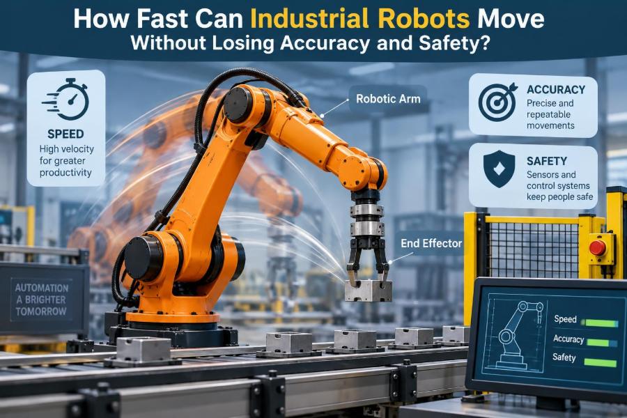
Industrial robots can move remarkably fast, yet “fast” is never a single number. It depends on the robot’s geometry, payload, tooling, path, controller settings, surrounding equipment, and the rules protecting people nearby.
The practical engineering question is not how fast a robot can move in an empty cell. It is how fast it can perform a specific task reliably, accurately, and safely over thousands of cycles.
🏁 Speed Is More Than a Top-Speed Specification
Robot datasheets often list maximum joint speeds or a maximum tool-center-point speed. Those values describe physical capability under defined conditions; they do not promise that every production path can run at that rate.
A robot rarely travels at a constant maximum speed. It must accelerate, decelerate, turn corners, stop at process points, avoid singular positions, and coordinate with machines, conveyors, or other robots. A short pick-and-place motion may spend more time accelerating and braking than cruising.
For production planning, cycle time is usually the more meaningful measure. It includes motion plus gripping, sensing, machine handshakes, inspection, and any dwell time required by the process.
🎯 Accuracy and Repeatability Are Different Measurements
Accuracy is how close the robot reaches the commanded position in the real world. Repeatability is how consistently it returns to the same position after repeated attempts.
A robot can be highly repeatable while having limited absolute accuracy. For example, it may place a part within a tight cluster that is slightly offset from the programmed location. In a fixed fixture, that can be acceptable; in off-line programmed work or large assembly, the offset may matter.
Speed can expose both problems. Dynamic forces, thermal changes, flexible tooling, and sensing delays can shift the actual path even when the controller reports that each axis followed its command closely.
📍 The Tool Center Point Defines What Actually Moves
The robot controller plans and controls a reference point called the tool center point, or TCP. It may be the tip of a welding torch, the center of a suction cup, or the point where a gripper contacts a part.
Changing an end effector changes the motion problem. A long welding torch magnifies small wrist rotations into larger tip movements. A wide gripper can sweep through more space than the robot flange, increasing collision risk even if the arm itself appears clear.
Correctly measuring the TCP and payload data is therefore a speed issue as much as a programming issue. Incorrect values can cause poor path tracking, unstable motion, and unreliable stopping behavior.
⚙️ Acceleration Usually Limits the Real Cycle Time
People often focus on velocity, but acceleration is frequently the stronger constraint. To go faster, a robot must build speed quickly and remove it quickly without exceeding motor torque, gearbox, structural, or payload limits.
Think of a car moving between closely spaced traffic lights. A higher top speed changes little if the driver must brake almost immediately. Similarly, a robot moving between nearby process points may gain more from tuned acceleration than from a larger velocity setting.
Aggressive acceleration can create overshoot, vibration, or excessive settling time. The shortest cycle is not always produced by the highest acceleration value; it is produced by the fastest motion that becomes stable when the tool reaches the next required point.
🧱 Payload Changes the Entire Motion Envelope
A robot’s rated payload is not merely a weight limit. It is tied to the payload’s center of gravity and moments of inertia, which describe resistance to rotational acceleration. A light but long workpiece can be harder to move than a compact heavier one.
When a robot carries a carton on extended forks, the payload acts like a lever. Sudden acceleration can bend the structure slightly, shift the box, or demand more torque from wrist joints. The robot may automatically limit performance, or a programmer may need to reduce speed manually.
- Verify mass, center of gravity, and inertia for every tool-and-part combination.
- Consider the worst case, such as a full tray rather than an empty one.
- Recheck values after changing grippers, hoses, cable packages, or product format.
🦾 Robot Geometry Makes Some Motions Easier Than Others
An articulated six-axis robot does not have the same dynamic capability everywhere in its workspace. A compact motion close to the base may use different joints and torque demands than a fully extended reach to the far side of a fixture.
At long reach, a robot can have less stiffness and more sensitivity to payload effects. A motion that runs smoothly near the center of the workspace may vibrate or lose positional margin at the edge.
This is why a single “safe speed” cannot be applied blindly across a whole program. Good cell design places critical, high-speed operations in favorable regions of the robot’s working envelope where practical.
🌀 Path Shape Controls Cornering Speed
A robot must slow for sharp changes in direction because its moving mass has momentum. The tighter the corner and the greater the required path fidelity, the less opportunity the controller has to blend motions smoothly.
In many programs, a fine or exact-stop instruction brings the robot to a precise point before the next move. A blended zone allows it to round the corner within a defined tolerance. Blending often shortens cycle time, but the TCP no longer passes through each programmed point exactly.
That trade-off is acceptable for a travel path above a conveyor. It may be unacceptable at a sealant start point, a connector insertion, or a laser-processing feature.
📏 Process Tolerance Sets the Useful Speed Limit
The robot’s motion requirements come from the process, not from its specification sheet. A robot transferring rough castings between bins can tolerate more path variation than one dispensing adhesive along a narrow bead path.
Welding, cutting, polishing, painting, force-controlled insertion, and vision-guided assembly each impose different limits on position, orientation, speed consistency, and timing. The correct question is: what variation can the product and downstream process actually accept?
Once that tolerance is defined, engineers can choose suitable path zones, acceleration profiles, sensing strategies, and verification methods. Without a tolerance target, “make it faster” is too vague to test responsibly.
🔩 Stiffness Determines How Much the Tool Deflects
No industrial robot is perfectly rigid. Links, joints, gearboxes, fixtures, tooling, and even the floor or pedestal have some compliance. Under changing loads, these elements deflect and recover.
This matters especially with long tools, heavy payloads, machining forces, or fast direction changes. The controller may place the flange correctly while the process tool at the TCP is still moving slightly relative to the part.
Better tooling design can sometimes improve performance more effectively than changing robot speed settings. Shorter load paths, rigid brackets, well-supported cable dress packs, and reduced overhang all help preserve usable accuracy.
📳 Vibration and Settling Can Erase Speed Gains
A robot can arrive at a target quickly yet still be unusable if the end effector oscillates afterward. This is called settling behavior. It is visible when a camera image blurs, a suction cup wobbles over a package, or a dispensing tip produces inconsistent starts and stops.
Increasing speed may reduce travel time but increase the wait required before a precise operation. The apparent improvement disappears if the program adds a longer dwell to let vibration decay.
Measure the whole sequence, including stabilization time. High-speed video, controller traces, vision data, and process-quality checks can reveal whether a motion is genuinely faster or simply moving the delay to another line of code.
🧠 The Controller Plans Motion Within Limits
Robot controllers coordinate all axes so the TCP follows a requested path while respecting configured velocity, acceleration, jerk, torque, and joint constraints. Jerk is the rate at which acceleration changes; limiting it can make motion smoother and reduce shocks.
The exact behavior depends on the manufacturer, robot model, and programming environment. A percentage speed override may scale motion, but it does not replace a review of individual moves, path tolerances, and system-level constraints.
Controllers can also apply automatic limits when payload data, joint position, singularity avoidance, or safety functions require them. Treat these interventions as information about the cell’s real capability, not merely as obstacles to bypass.
🔄 Joint Speed Is Not the Same as TCP Speed
Each robot axis rotates or translates according to its own kinematics. The TCP speed produced by those axis motions changes with robot posture. A modest wrist movement may create a fast tool-tip sweep when the tool is long.
Conversely, holding a straight Cartesian path at a constant TCP speed may demand very different joint speeds along the route. Near difficult postures, one joint can become the limiting axis even though the requested TCP speed looks reasonable.
This distinction matters when diagnosing slow programs. The remedy may be a different approach orientation or intermediate point, not simply a larger global speed command.
🧭 Singularities Create Awkward High-Speed Regions
A singularity is a robot configuration where small TCP movements can require extremely large changes in one or more joint angles, or where the robot loses a degree of directional freedom. Wrist alignment is a common example on six-axis arms.
Near a singularity, the controller may slow the robot, alter joint behavior, or issue a warning. Passing through one at speed can cause abrupt axis motion, poor path quality, or unpredictable orientation behavior depending on the task and controller strategy.
Program paths to avoid problematic configurations where possible. Changing the robot’s elbow posture, rotating the tool slightly, or moving an approach point can preserve both cycle time and control quality.
🧰 End Effectors Often Become the Bottleneck
The robot is only one moving part of an automated cell. Pneumatic grippers need air flow and time to close; vacuum tools need time to establish a reliable seal; mechanical clamps may require confirmation from sensors.
At high acceleration, a part may slip in the gripper or deform under suction. A gripper that works during a slow demonstration may fail intermittently in production because it was never validated against the actual inertial loads.
Tool selection should match the intended acceleration and orientation changes. Grip force, friction, suction area, valve response, part geometry, and detection logic all shape the safe performance limit.
📦 Product Behavior Can Be Less Predictable Than the Robot
Rigid metal components behave differently from flexible pouches, loose bags, open containers, wet parts, and stacked products. A robot may repeat its trajectory precisely while the item it carries shifts, swings, spills, or catches air.
For example, rapidly moving an open tray of small components can create internal movement that defeats otherwise accurate placement. A high-speed palletizing path can make unstable loads lean even when each individual pick is successful.
Test with representative product conditions, including variation in mass, surface finish, fill level, temperature, and packaging. The fastest reliable setting is often established by the product’s behavior, not the arm’s rated capacity.
👁️ Vision Systems Add Timing and Uncertainty
Machine vision can let a robot locate randomly oriented parts, inspect features, or track a moving conveyor. But image exposure, processing, communication, and coordinate transformation all introduce timing considerations.
If a part is moving, the system must account for where it will be when the robot reaches it, not only where it was when the image was taken. Conveyor tracking functions are designed for this task, but their quality depends on calibration, encoder signals, camera setup, and predictable part motion.
Moving the robot faster may leave less time for a new image or correction. Fast handling and robust vision work well together when the total timing budget is designed explicitly.
⏱️ Synchronization Limits Cell Throughput
A robot that finishes early may still wait for a machine door, a conveyor index, a barcode read, a safety reset, or another robot sharing the workspace. Raising its motion speed will not improve line output if another stage controls the bottleneck.
Map the cycle as a sequence of dependencies. Look for actions that can occur in parallel, such as beginning a camera exposure while a gripper releases, but do not overlap motions that compromise access or safety.
This broader view avoids a common error: optimizing a robot path in isolation while creating more waiting, congestion, or inconsistent handoffs elsewhere in the cell.
🛑 Safety Functions Intentionally Constrain Motion
Industrial robot safety is not a separate feature added after speed optimization. It defines where, when, and how the robot may move. Safeguards can include perimeter fencing, interlocked gates, presence-sensing devices, enabling devices, safety-rated monitored stops, and reduced-speed modes.
When people can enter or share a space with a robot, risk assessment determines appropriate protective measures. The design must consider hazards from the robot, tooling, payload, pinch points, ejected parts, stored energy, and connected machinery.
Never treat a safety slowdown as an arbitrary productivity loss. It may be the engineered response to a person entering a zone where separation distance or stopping performance matters.
🚧 Stopping Distance Matters as Much as Running Speed
A faster robot generally needs more distance and time to stop, although the relationship depends on the robot, payload, direction, braking system, and configured safety function. Protective devices must be positioned with stopping performance and detection timing in mind.
Safety design therefore cannot rely on a nominal maximum speed alone. A safety engineer evaluates the actual system behavior, including response times from sensors, safety logic, drives, brakes, and the moving mechanism.
Any change to payload, speed, path, tooling, or guard layout can affect the assumptions behind that design. Changes should be reviewed through the site’s machinery-safety process rather than adjusted casually at the teach pendant.
🤝 Collaborative Operation Does Not Mean Unlimited Speed
Collaborative robot applications are often misunderstood as inherently safe at any speed. A collaborative application is defined by how risks are managed, which may involve power-and-force limiting, speed-and-separation monitoring, hand guiding, safety-rated monitored stop, or other protective strategies.
A robot designed for collaborative use can still create hazards through sharp tools, heavy payloads, crushing zones, or a moving workpiece. Its permitted speed may change according to separation from people and the task’s assessed contact risks.
The useful distinction is simple: collaboration is a system-level safety design, not a license to eliminate guarding or skip risk assessment.
🧪 Validate at Production Conditions, Not Just in Simulation
Offline simulation is valuable for reach studies, collision checks, approximate cycle estimates, and layout decisions. However, a simulation may not fully capture flexible cables, part variation, pneumatic response, floor vibration, calibration error, or real controller behavior.
Commissioning should use a structured ramp-up. Start with conservative motion settings, confirm clearances and safety functions, then increase performance while monitoring quality, grip reliability, motor load, faults, and actual cell cycle time.
Record the tested configuration. A program proven with one product, tool, and payload may need revalidation after a seemingly minor mechanical or process change.
📈 Measure the Right Performance Signals
Cycle time is essential, but it is not enough. A high-speed setting that creates occasional missed picks, poor weld quality, dropped parts, or frequent recovery routines may reduce total output over a shift.
Useful measures combine motion and process results:
- completed good parts per unit time, rather than commanded cycle time alone;
- position or process-quality variation at critical features;
- gripper confirmation failures, vision retries, and controller alarms;
- unplanned stops and the time needed to recover safely;
- wear indicators in tooling, cables, fixtures, and mechanical components.
A stable setting with a slightly longer nominal cycle can outperform an aggressive setting that repeatedly interrupts production.
🛠️ Path Optimization Often Beats Raising the Override
Before increasing global speed, remove unnecessary distance. A poorly planned path may lift too high, travel around empty space, stop at points that do not require exact positioning, or use inefficient robot configurations.
Useful improvements include reducing clearance where risk assessment and process needs allow, using blended travel moves away from critical operations, choosing favorable approach angles, and reorganizing tasks to reduce backtracking.
These changes should be reviewed for collisions, cable movement, access, and safety zones. The goal is not simply a shorter programmed route; it is a shorter route that remains robust against normal variation.
🧩 Mechanical Cell Design Sets a Ceiling
Robot speed cannot compensate for a weak fixture, unstable pedestal, poor part presentation, or cramped layout. Mechanical design determines repeatable datum locations, clear access, cable routing, and the amount of motion required per cycle.
A fixture that locates a part reliably can reduce the need for slow search routines or complex vision corrections. A well-positioned infeed can eliminate a long robot reach. These upstream improvements often create durable gains because they simplify every future cycle.
When designing a new cell, involve controls, safety, manufacturing, tooling, and maintenance teams early. Their constraints are interconnected long before the robot is powered on.
🔧 Maintenance Preserves High-Speed Performance
Fast, repetitive motion places demand on cables, dress packs, grippers, bearings, reducers, and fixtures. Wear does not always appear as an immediate robot fault; it may first show up as drifting quality, increased vibration, or intermittent sensor problems.
Inspect routed hoses and cables for rubbing and fatigue, verify fixture fasteners, clean sensors, check gripper condition, and follow the manufacturer’s maintenance requirements. Monitor changes rather than waiting for a complete failure.
A speed setting that was acceptable at launch may need reassessment if the tool is modified, the product changes, or maintenance evidence shows reduced mechanical margin.
⚠️ Common Speed-Optimization Mistakes
Several tempting shortcuts create fragile automation. They may make a short demonstration look impressive while increasing downtime or risk over sustained production.
- Using a global speed override as the main optimization tool: it ignores path-specific and process-specific constraints.
- Copying settings from another cell: a different payload, reach, tool, or safety layout can change the outcome completely.
- Testing with empty tooling: the actual part may introduce inertia, slip, deflection, or variability.
- Reducing safety margins to remove nuisance stops: nuisance stops should be investigated, not defeated.
- Judging success by one clean cycle: robust settings must survive normal shifts, product variation, and recovery conditions.
🧭 A Practical Method for Finding the Right Speed
Start by identifying the process-critical points: pickup, placement, contact, inspection, dispensing, machine loading, and any location near people or equipment. Define what each point requires in position, orientation, speed, and dwell.
- Verify payload, TCP, tool geometry, calibration, and safeguarding assumptions.
- Measure the baseline cycle and identify the real bottleneck.
- Optimize path distance and blending in noncritical travel segments.
- Increase speed or acceleration in controlled increments.
- Check product quality, grip stability, clearances, stops, and recovery behavior at each increment.
- Document the accepted settings and change-control conditions.
This approach turns “go faster” into an engineering experiment with observable acceptance criteria.
🏭 Different Applications Have Different Speed Priorities
| Application | What commonly limits speed | Typical optimization focus |
|---|---|---|
| Machine tending | Door timing, chuck confirmation, machine cycle | Coordinate handshakes and reduce robot travel during machine time |
| Palletizing | Payload inertia, load stability, gripper behavior | Efficient layers, smooth acceleration, stable load patterns |
| Arc welding | Weld quality, seam tracking, torch path consistency | Stable process speed and accurate starts, stops, and orientation |
| Dispensing | Bead geometry, pressure response, corner behavior | Consistent TCP speed and controlled transitions |
| Assembly | Part tolerance, insertion force, sensing | Fast approach followed by slower, verified contact motion |
The pattern is consistent: the fastest sections of a program are usually the low-risk travel sections, while critical process interactions are deliberately controlled.
🧑🏫 What Programmers and Operators Should Communicate
Speed changes affect more than robot code. Operators may notice new product movement, maintenance technicians may see cable wear, and quality staff may detect subtle variation before a robot fault appears.
Clear communication should state what changed, why it changed, the approved payload and product range, expected behavior, and the conditions that require escalation. A documented baseline makes it easier to distinguish normal variation from an emerging issue.
For students and newer engineers, this is an essential lesson: industrial automation is a multidisciplinary system. Strong robot programming includes listening to evidence from the people who run and maintain the cell.
🌟 The Core Principle: Fast Enough Is a System Decision
Industrial robots can be extremely fast, but no honest answer can be reduced to one maximum velocity. Useful speed emerges from the interaction of dynamics, path geometry, payload, tooling, process tolerance, synchronization, and safeguarding.
The best-performing cell is not necessarily the one whose robot arm looks fastest. It is the one that produces good parts consistently, avoids unsafe conditions, recovers predictably, and maintains its performance over time.
When evaluating any proposed speed increase, ask four questions: Does it improve throughput at the bottleneck? Does it preserve process quality? Does it remain reliable with real products? Does it remain within the validated safety design? If any answer is uncertain, the next step is measurement and review, not a larger override.
Industrial robot speed is valuable only when accuracy, product control, and safety move forward with it. That is how a fast motion becomes dependable automation rather than a recurring source of downtime. 🦾🎯🛑