
When a warehouse robot carries a package across a fulfillment center, a self-driving vehicle navigates around traffic, or a robotic vacuum moves through a home, the machine must solve an important problem:
How can I get from where I am now to where I need to go without hitting anything? 🗺️🤖
This challenge is known as path planning.
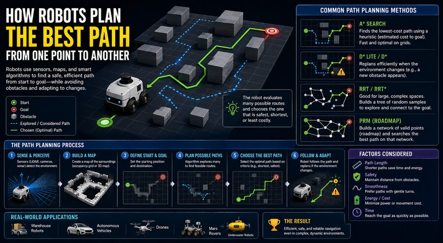
Path planning is the process of finding a safe and practical route between a robot’s starting position and a destination. Depending on the application, the “best” path might mean the shortest route, the fastest route, the path that uses the least energy, or the route with the lowest risk of collision.
A simplified planning process looks like:
Know current position ➡️ understand surroundings ➡️ identify obstacles ➡️ search possible routes ➡️ choose path ➡️ move while continuously checking conditions
Although humans perform similar reasoning almost automatically when walking through a room, robots must convert the problem into mathematics, geometry, algorithms, and sensor measurements. 🧠📐
🗺️ Step 1: The Robot Needs a Representation of Its Environment
Before a robot can plan a route, it needs some understanding of the space around it.
This representation is commonly called a map.
A map may contain:
- Walls
- Furniture
- Roads
- Shelves
- Doors
- Obstacles
- Restricted areas
- Traversable surfaces
Different robots use different kinds of maps.
A warehouse robot may have a detailed digital map of every aisle.
A robotic vacuum may construct its map while exploring a home.
A self-driving vehicle may combine detailed road maps with real-time sensor data.
The map essentially tells the planning system:
These areas are free ➡️ movement is possible
These areas are occupied ➡️ avoid them
🧱 Occupancy Grids Turn Space Into Cells
One common mapping method is an occupancy grid.
The environment is divided into many small squares or cells.
Each cell may be classified as:
Free ✅
Occupied ❌
Unknown ❓
Imagine a floor plan represented as a large digital chessboard.
If a wall passes through a cell, that cell is marked as occupied.
If the robot has confirmed that a cell is empty, it is marked as free.
The planning algorithm then searches for a sequence of free cells connecting the robot’s location with its destination.
Smaller cells provide more detail but require more memory and computation.
This creates a trade-off between map accuracy and processing speed. ⚙️
📍 Step 2: The Robot Must Know Where It Is
A map is useless if the robot does not know its own position within it.
This challenge is called localization.
A robot may estimate its position using:
- Wheel encoders
- Cameras 📷
- Lidar
- GPS 🛰️
- Radar
- Inertial sensors
- Ultrasonic sensors
- Known landmarks
A warehouse robot might determine that it is located at coordinates:
(x = 12.4 m, y = 8.1 m)
and oriented:
35° relative to the map
Once the robot knows:
Current position + destination
the path planner can begin searching.
🧭 SLAM Helps Robots Map and Localize Simultaneously
Sometimes a robot enters an environment without a complete map.
In this case, it may use a technique called Simultaneous Localization and Mapping, or SLAM.
SLAM attempts to solve two problems at once:
Where am I?
and:
What does the environment look like?
The robot moves, observes walls or landmarks, estimates its motion, and gradually builds a map while refining its own position.
This technology is widely used in:
🏠 Robot vacuums
🏭 Mobile industrial robots
🚗 Autonomous vehicles
🚁 Drones
🧪 Research robots
Once enough of the environment has been mapped, conventional path-planning algorithms can use that map.
🔍 The Central Problem: Search Through Possible Routes
A robot may have thousands, millions, or even infinitely many possible ways to reach a destination.
Trying every possible path would be inefficient.
Path-planning algorithms therefore search the environment intelligently.
A basic path-planning problem consists of:
Start: Robot’s current location
Goal: Desired destination
Obstacles: Areas that cannot be entered
Cost: A measure of how desirable each possible route is
The algorithm searches for a route that minimizes the chosen cost.
📏 What Does “Best Path” Actually Mean?
The shortest geometric path is not always the best.
A robot may need to optimize several factors.
Possible goals include:
- Minimum distance 📏
- Minimum travel time ⏱️
- Minimum energy use 🔋
- Maximum clearance from obstacles
- Smooth turns
- Minimum wheel wear
- Avoidance of dangerous areas
- Reduced congestion
A hospital delivery robot, for example, might prefer a slightly longer hallway if the shorter route passes through a crowded emergency area.
The planner converts these preferences into a cost function.
Conceptually:
Path cost = distance + obstacle risk + turning cost + other penalties
The route with the lowest total cost becomes the preferred solution.
🧮 Dijkstra’s Algorithm
One classic route-search method is Dijkstra’s algorithm.
The algorithm treats the environment like a graph consisting of:
Nodes ➡️ possible positions
Edges ➡️ allowed movements
Each movement has a cost.
Dijkstra’s algorithm begins at the starting point and gradually explores outward.
It always investigates the currently known location with the lowest accumulated cost.
Eventually, it reaches the goal.
One important property is that, when edge costs are nonnegative, Dijkstra’s algorithm can find the lowest-cost path.
However, it may explore many locations that are not particularly useful because it does not inherently know which direction the destination lies. 🗺️
⭐ A* Search Makes Planning More Efficient
A very popular robot path-planning algorithm is A*, pronounced “A-star.”
A* improves on basic shortest-path search by using an estimate of how far each candidate location is from the goal.
Its evaluation function is commonly written:
f(n) = g(n) + h(n)
where:
- g(n) = cost from the starting point to node
n - h(n) = estimated cost from node
nto the goal - f(n) = estimated total route cost
The function h(n) is called a heuristic.
For example, the algorithm might estimate the remaining distance using straight-line distance.
A* therefore asks:
How expensive has this route been so far?
plus:
How promising does it look from here to the destination?
This helps the search focus toward the goal instead of exploring equally in every direction. 🎯
📐 Why the Heuristic Matters
Imagine a robot trying to reach a charging station located northeast of its current location.
Without a heuristic, the planner may search many cells to the southwest, west, and south.
A useful heuristic tells the algorithm:
The destination is probably in this direction.
The heuristic must be selected carefully.
If it is appropriately designed, A* can still find an optimal path while exploring significantly fewer possibilities than uninformed search.
Common heuristics include:
- Manhattan distance
- Euclidean distance
- Diagonal distance
The correct choice depends on how the robot is allowed to move.
🧭 Manhattan Versus Euclidean Distance
Suppose a robot moves on a square grid.
If it can move only:
⬆️ Up
⬇️ Down
⬅️ Left
➡️ Right
then Manhattan distance may be appropriate.
It is calculated using:
|x₁ – x₂| + |y₁ – y₂|
If the robot can travel more freely in arbitrary directions, Euclidean distance may be more suitable.
That is the familiar straight-line distance:
√[(x₂-x₁)² + (y₂-y₁)²]
These mathematical estimates help the planner judge which candidate positions are most promising.
🌳 Rapidly-Exploring Random Trees
Grid-based algorithms are excellent in many environments, but some robotic systems operate in continuous spaces with complex movement constraints.
For these applications, planners may use algorithms such as Rapidly-Exploring Random Trees, commonly abbreviated as RRT.
RRT works by repeatedly sampling random locations in the robot’s configuration space.
The algorithm builds a branching tree extending outward from the starting state.
A simplified process is:
Start node ➡️ sample random point ➡️ extend tree toward point ➡️ reject collisions ➡️ repeat
Over time, the tree spreads through open regions.
When one branch approaches the goal, the planner can extract a path.
RRT-based methods are particularly useful for robotic arms and systems with complex geometry. 🌳🤖
🦾 Robot Arms Need to Plan More Than Position
A mobile robot moving across a floor may be represented mainly by:
x position + y position + orientation
A robotic arm is more complicated.
A six-joint industrial robot may need to consider six joint angles simultaneously.
Its state might look like:
q = (θ₁, θ₂, θ₃, θ₄, θ₅, θ₆)
Every possible combination of joint positions represents a point in a high-dimensional configuration space.
The planner must find a sequence of joint configurations that moves the robot’s hand to the target while ensuring that:
- The arm does not hit itself
- The arm avoids nearby machines
- Joint limits are respected
- Motion remains physically achievable
This is one reason motion planning for robotic manipulators can be computationally challenging.
🚧 Robots Must Account for Their Own Size
A path that is safe for a single mathematical point may not be safe for a physical robot.
Imagine a narrow opening 50 centimeters wide.
If the robot is 80 centimeters wide, it cannot pass through.
Planning systems therefore incorporate the robot’s physical dimensions.
One common technique is obstacle inflation.
Instead of modeling the full robot shape at every calculation, obstacles are enlarged by a safety margin.
The robot can then sometimes be treated approximately as a point traveling through the remaining free space.
Conceptually:
Real obstacle + robot radius + safety margin = inflated obstacle
This greatly simplifies collision checking. 🧱
🛡️ Safety Margins Prevent Near-Collisions
Robots generally should not travel millimeters away from walls merely because the geometry technically allows it.
Localization errors, wheel slip, sensor noise, and moving objects create uncertainty.
Planners therefore add clearance costs.
A location close to a wall might be allowed but assigned a high cost.
A path through the middle of an open corridor receives lower risk cost.
The planner may therefore choose:
Slightly longer + safer
instead of:
Shortest + dangerously close to obstacles
This creates more robust real-world behavior.
🌍 Global Planning Versus Local Planning
Robotic navigation is often divided into two levels.
🗺️ Global Planner
The global planner calculates the overall route from start to destination using a relatively large map.
For example:
Warehouse station A ➡️ aisle 4 ➡️ corridor 2 ➡️ loading dock
🚧 Local Planner
The local planner handles immediate motion.
It reacts to nearby obstacles and determines commands such as:
- Turn slightly left
- Reduce speed
- Stop
- Move around pedestrian
This division is important because the world can change after the global route is calculated.
🚶 Dynamic Obstacles Require Real-Time Reaction
A static map may show walls and furniture, but many environments contain moving obstacles:
- People
- Cars
- Forklifts
- Other robots
- Animals
Suppose the global planner calculates a perfect route through a hallway.
Seconds later, a person steps into the path.
The robot cannot blindly follow its original plan.
Its sensors detect the obstacle, and the local planner modifies the motion.
Possible responses include:
Slow down ➡️ wait
or:
Move around obstacle
or:
Recalculate the entire route
This is known as dynamic replanning. 🔄
🔄 Replanning When the World Changes
Imagine a warehouse robot discovers that an aisle has been blocked by a pallet.
The original route may no longer be valid.
The system updates its map:
Previously free cell ➡️ now occupied
The planner then searches for another route.
Modern robots may perform this replanning continuously.
This allows them to adapt to environments that differ from their original maps.
Algorithms such as D* and related incremental search methods are designed to update routes efficiently when map information changes.
🚗 Vehicles Need Paths That Are Physically Drivable
A simple grid planner might produce a path containing abrupt 90-degree turns.
A small omnidirectional robot may be able to follow such a path.
A car cannot.
Cars have steering limits and minimum turning radii.
Autonomous-vehicle planners therefore account for kinematic constraints.
The route must satisfy conditions such as:
- Maximum steering angle
- Vehicle width
- Turning radius
- Direction of motion
- Acceleration limits
A geometrically short route may be rejected because the vehicle cannot physically execute it.
🌊 Path Smoothing
Search algorithms often initially produce paths consisting of many straight-line segments or grid steps.
These may be mathematically valid but mechanically inefficient.
A path smoothing stage can convert a jagged path into smoother curves.
For example:
Raw route: sharp zigzag pattern
Smoothed route: gradual continuous curve
Smoother paths offer several benefits:
- Lower mechanical stress
- Less energy use
- Higher passenger comfort
- Easier control
- Faster travel
Autonomous vehicles and drones especially benefit from smooth trajectories.
⏱️ Path Planning Versus Trajectory Planning
A path describes where the robot should travel.
A trajectory also describes when the robot should be at each location.
Path:
A ➡️ B ➡️ C
Trajectory:
A at 0 seconds ➡️ B at 4 seconds ➡️ C at 8 seconds
Trajectory planning therefore includes:
- Velocity
- Acceleration
- Timing
- Sometimes jerk, which is the rate of change of acceleration
Industrial robots need carefully timed trajectories so their motors move smoothly and remain within force and speed limits.
🔋 Energy Can Influence the Route
For battery-powered robots, the shortest route is not always the most energy-efficient.
Consider two paths.
Path A: Short but steep uphill
Path B: Longer but relatively flat
A delivery robot may use less energy on Path B.
Energy-aware planners can consider:
- Terrain slope
- Motor effort
- Acceleration
- Surface type
- Battery level
A drone may also consider wind conditions.
Flying directly against strong wind may use more energy than taking a longer route with favorable airflow.
🚁 Drones Add a Third Dimension
Ground robots often plan mainly in two dimensions.
Drones navigate through three-dimensional space.
Their state may include:
x, y, z position + orientation + velocity
Obstacles may include:
🏢 Buildings
🌳 Trees
⚡ Power lines
🚁 Other aircraft
⛰️ Terrain
A drone path planner must also account for flight dynamics, wind, restricted airspace, battery capacity, and landing options.
Three-dimensional planning dramatically increases the number of possible routes.
🚚 Multiple Robots Need Coordinated Planning
Warehouses may contain hundreds of mobile robots operating simultaneously.
If every robot simply chooses its own shortest path, they may block one another.
Imagine two robots entering the same narrow aisle from opposite directions. 🚧
The system therefore needs multi-agent path planning.
It may reserve regions of space for particular times.
For example:
Robot A uses intersection at 10:01:05
Robot B waits until 10:01:08
The planner is now optimizing both:
Space + time
This helps prevent collisions and traffic jams.
🚦 Traffic Management for Robot Fleets
Large robot fleets may use central traffic-management software.
The system can:
- Assign destinations
- Reserve routes
- Prevent intersection conflicts
- Balance congestion
- Prioritize urgent jobs
A route that is physically shortest may be avoided because too many robots are already using it.
The planner might choose a longer but less congested corridor.
This is remarkably similar to navigation apps rerouting cars around traffic. 🚗📱
📡 Sensors Continuously Verify the Plan
A path planner relies on maps and estimates, but sensors verify what is actually happening.
Common navigation sensors include:
🔦 Lidar
Measures distance using laser pulses.
📷 Cameras
Identify objects, lanes, markers, and visual landmarks.
📡 Radar
Measures distance and relative motion, especially useful for vehicles.
🔊 Ultrasonic Sensors
Useful for detecting nearby objects.
🛰️ GPS
Provides global position outdoors.
🧭 IMU
Measures acceleration and rotational motion.
Combining these measurements helps the robot understand whether it is still following the planned path correctly.
🧠 Cost Maps Help Combine Many Concerns
Modern navigation systems often use a cost map.
Instead of classifying every location as simply free or blocked, the map assigns numerical costs.
For example:
Open space: cost 1
Near wall: cost 10
Rough terrain: cost 20
Restricted zone: cost 100
Obstacle: infinite cost
The planner searches for the route with the lowest total accumulated cost.
This makes it possible to encode many practical preferences inside one mathematical framework. 📊
⚠️ Planning Must Handle Uncertainty
Robotic measurements are never perfectly accurate.
A sensor might report a wall at:
5.02 meters
when its true distance is:
5.00 meters
Wheel slip can also cause localization errors.
Robust planning systems therefore account for uncertainty.
They may:
- Increase obstacle margins
- Reduce speed in uncertain areas
- Maintain backup routes
- Replan frequently
- Use probabilistic maps
Safety-sensitive robots usually favor reliable behavior over the absolute theoretical shortest route.
🤖 Machine Learning Can Complement Classical Planning
Traditional path-planning algorithms such as A*, Dijkstra, and RRT rely heavily on explicit mathematical rules.
Machine learning can complement these methods.
For example, learned systems may:
- Predict pedestrian movement
- Estimate terrain difficulty
- Identify navigable regions from camera images
- Predict traffic congestion
- Suggest promising route candidates
However, many real robots still use classical planning algorithms because their behavior is structured, interpretable, and mathematically well understood.
A practical robotic system may combine:
Machine learning for perception ➡️ classical algorithms for planning ➡️ control algorithms for motion
🎛️ Planning Is Different From Control
Once a path is calculated, another system must actually make the robot follow it.
This is the job of the motion controller.
Suppose the planned path curves left.
The controller determines the motor commands needed to follow that curve.
For a wheeled robot, it may adjust:
- Left-wheel speed
- Right-wheel speed
- Steering angle
The architecture becomes:
Perception ➡️ localization ➡️ path planning ➡️ trajectory planning ➡️ motor control
Each stage solves a different part of the navigation problem.
🧪 Simulation Helps Engineers Test Planning Algorithms
Before deploying navigation software on expensive hardware, engineers often test it in simulation.
A simulated environment can contain:
- Walls
- Moving pedestrians
- Vehicles
- Sensor noise
- Slippery surfaces
Engineers can then test thousands of scenarios.
For example:
What happens if a pedestrian suddenly blocks the route?
Can the planner escape a dead end?
Does the robot avoid narrow unsafe gaps?
Simulation allows difficult and potentially dangerous situations to be tested without damaging equipment or putting people at risk. 💻
🏭 Real-World Applications of Robot Path Planning
Path planning appears in many industries.
📦 Warehouses
Robots move inventory between storage shelves and packing stations.
🚗 Autonomous Vehicles
Cars plan routes through road networks and around nearby obstacles.
🏠 Robot Vacuums
Cleaning robots navigate rooms while avoiding furniture.
🦾 Manufacturing
Robot arms plan collision-free motions around machinery.
🚁 Drones
Aircraft plan three-dimensional routes around obstacles and restricted regions.
🏥 Hospitals
Delivery robots transport medicine, meals, and supplies through corridors.
🌾 Agriculture
Autonomous machines plan efficient paths through fields.
The underlying mathematical challenge is similar even though the environments differ.
🧭 A Simplified Robot Navigation Example
Imagine a delivery robot in an office building.
Its goal is to travel from the mailroom to Room 310.
The process might look like this:
1. Localize itself. 📍
The robot determines that it is in the mailroom.
2. Load the map. 🗺️
The system identifies corridors, walls, doors, and elevators.
3. Set destination. 🎯
Room 310 becomes the goal.
4. Build a cost map.
Walls are blocked, narrow areas receive higher cost.
5. Run A.* ⭐
The planner finds a low-cost route.
6. Smooth the route.
Sharp turns are converted into manageable curves.
7. Begin driving. 🤖
The controller follows the trajectory.
8. Detect a person blocking the hallway. 🚶
The local planner slows or moves around them.
9. Discover a closed corridor. 🚧
The global planner recalculates another route.
10. Reach Room 310. ✅
What looks like ordinary navigation is actually a continuous cycle of sensing, estimation, planning, prediction, and control.
🏁 Conclusion
Robot path planning is the process of finding a safe and useful route from a starting location to a destination. 🤖🗺️
To do this, the robot must first understand its surroundings and estimate where it is.
The planner then represents possible movements mathematically and searches for a route around obstacles.
Algorithms such as Dijkstra’s algorithm can find minimum-cost routes, while A* uses heuristics to search more efficiently toward the destination.
For complex continuous spaces, algorithms such as RRT can explore possible motions without requiring a simple grid.
But finding the shortest route is only part of the problem.
Real robots must also consider:
Obstacle clearance + turning limits + energy + traffic + moving objects + uncertainty + physical dynamics
A global planner may find the overall route, while a local planner handles immediate obstacles.
If the environment changes, the robot can replan.
Once the route is selected, trajectory and motor-control systems convert that abstract path into real movement.
The entire process can be summarized as:
Map the world ➡️ know your position ➡️ evaluate possible routes ➡️ choose the best one ➡️ move ➡️ sense changes ➡️ replan when necessary. 🔄
Whether it is a warehouse robot avoiding shelves, a drone navigating between buildings, or an autonomous vehicle steering through traffic, successful navigation depends on continuously answering the same fundamental question:
“Given where I am, where I want to go, and what stands in the way, what is the safest and most efficient route forward?” 🚀🤖