
A robot arm picks up a part from a conveyor, rotates its wrist, and places the part into a tray. To a person, the motion looks obvious: reach there, turn this way, release.
For the robot, that apparently simple move is a geometry problem, a control problem, and sometimes a puzzle with several valid answers. Its motors do not directly understand “move the gripper to the tray.” They move individual joints.
Kinematics gives robots the mathematical language needed to connect those joint motions to a physical position and orientation in space. It is what turns motor angles into a predicted tool location—and a desired tool location into a set of motor commands.
Those two directions are called forward kinematics and inverse kinematics. They appear in industrial arms, collaborative robots, camera gimbals, humanoids, animation rigs, surgical systems, and mobile manipulators.
🧭 The central question kinematics answers
Kinematics describes motion through geometry: positions, orientations, velocities, and accelerations. It deliberately begins without asking what forces, torques, masses, or friction are involved.
For a robot manipulator, the central relationship is between its joint space and its task space. Joint space contains variables such as motor angles and linear slide positions. Task space describes where the end tool is and which way it faces.
Dynamics comes later, when engineers calculate how much torque is required to execute a motion. A robot generally needs both kinematics and dynamics, but they solve different questions.
🦾 Robot arms are chains of links and joints
A serial robot arm is built from rigid pieces called links, connected by joints. Each independently controllable joint contributes a degree of freedom, often abbreviated as DOF.
A revolute joint rotates, like an elbow. A prismatic joint translates along an axis, like a telescoping rail. A six-axis industrial arm commonly combines six revolute joints so its tool can reach a position and choose an orientation.
The end of the chain is the end effector: perhaps a gripper, welding torch, suction cup, camera, or screwdriver. Kinematic calculations often track a convenient point and coordinate frame on that tool, called the tool center point (TCP).
📍 Position and orientation are different requirements
Specifying a target point such as “300 millimeters forward and 200 millimeters left” only defines position. A gripper also needs an orientation: its approach direction and rotational alignment.
Consider inserting a key into a lock. The key must reach the lock’s location, but it must also face the correct way and be rotated to match the slot. The same distinction matters when placing circuit boards, applying sealant, or welding along a path.
In three-dimensional work, a tool pose usually means three position values plus three orientation values. Engineers may represent orientation with rotation matrices, Euler angles, axis-angle notation, or quaternions, depending on the task.
➡️ Forward kinematics: joints in, pose out
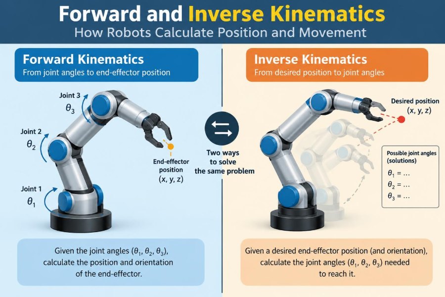
Forward kinematics (FK) starts with known joint variables and calculates the resulting pose of the end effector. If encoders report every joint angle, FK predicts where the robot’s tool should be.
For a simple two-link planar arm, if the shoulder angle is q₁ and elbow angle is q₂, with link lengths L₁ and L₂, the endpoint is:
x = L₁ cos(q₁) + L₂ cos(q₁ + q₂)
y = L₁ sin(q₁) + L₂ sin(q₁ + q₂)
The second link’s direction depends on both angles because the elbow rotates relative to the first link. This accumulation of transformations is the essential pattern behind larger robot models.
🔗 Why transformations are chained together
Every link has its own local coordinate frame. Moving from the base to the first link, then to the second link, and finally to the tool means applying a sequence of rotations and translations.
Each transformation says, in effect, “where is the next frame relative to the current one?” Multiplying them in the correct order produces the tool frame relative to the robot base.
This modular approach is valuable because it works for many mechanisms. Add a wrist, a tool adapter, or an external linear axis, and the chain can be extended rather than reinvented.
🧮 Homogeneous matrices keep geometry organized
Robotics commonly uses a 4×4 homogeneous transformation matrix to store a 3D rotation and translation together. It lets engineers combine successive coordinate-frame changes with ordinary matrix multiplication.
T = [ R  p ]
    [ 0  1 ]
Here, R is a 3×3 rotation matrix and p is a three-value position vector. A chain from base to tool may be written as T₀ᵀ = T₀¹T₁²…Tₙᵀ.
The notation can look abstract at first, but it prevents a frequent error: mixing up a point expressed in one coordinate frame with the same physical point expressed in another.
📐 Coordinate frames make robot instructions unambiguous
A coordinate frame assigns an origin and three perpendicular axes. Robots usually use at least a base frame, a frame for each joint or link, a tool frame, and often a workpiece or camera frame.
“Move 50 millimeters in X” has no useful meaning until the frame is named. Moving in the base X direction may differ greatly from moving in the tool’s own X direction after the wrist has rotated.
Good frame management is also essential for vision-guided work. A camera can identify an object in camera coordinates, but the robot needs that target converted reliably into its base or workcell coordinates.
🧱 Kinematic conventions reduce modeling ambiguity
To create a repeatable model, engineers attach frames according to a convention. The classic method is the Denavit–Hartenberg (DH) convention, which describes adjacent links using geometric parameters such as link length, link twist, joint offset, and joint angle.
DH tables are compact and widely taught, but frame assignment can be easy to misapply, especially around parallel or intersecting axes. Modified DH conventions use a different ordering and should not be mixed casually with standard DH formulas.
Modern software may define transforms directly from CAD geometry or use product-of-exponentials formulations. The best representation is the one that matches the robot model, team tools, and calibration process clearly.
🧪 A two-link arm reveals the whole idea
Imagine a tabletop arm with two 1-meter links. With both joints at zero and its reference direction along positive X, the endpoint lies 2 meters from the base. Rotate the shoulder by 90 degrees, and the same arm points upward instead.
Now bend the elbow while holding the shoulder fixed. The tip traces a circle centered at the elbow, not at the base. Forward kinematics captures that result automatically because each downstream transform inherits the upstream rotations.
This small example scales conceptually to a six-axis arm. The arithmetic becomes larger, but the rule remains: start at the base and compose each joint-and-link transformation in order.
🔄 Inverse kinematics: pose in, joints out
Inverse kinematics (IK) reverses the question. Given a desired tool pose, it seeks joint values that place the tool at that pose.
IK is what makes a high-level command practical. A programmer may define a target pose over a fixture, while the controller determines shoulder, elbow, and wrist angles that could achieve it.
Unlike FK, IK is not always a single clean calculation. A target can have several solutions, no solution, or solutions that are technically correct but operationally poor.
🧩 One target can have multiple arm configurations
For the planar two-link arm, many reachable points can be achieved with an “elbow-up” or “elbow-down” posture. Both place the endpoint at the same location, but the links sweep through different parts of the workspace.
A six-axis arm can offer additional branches: shoulder left or right, elbow high or low, and wrist flipped or unflipped. Manufacturers often expose configuration settings so a program can request a consistent posture.
Choosing among valid solutions matters. One route may avoid a fixture, preserve cable clearance, keep joints away from their limits, or make the next move shorter and smoother.
🚫 Some requested poses are unreachable
A target beyond the arm’s maximum reach has no IK solution. So does a pose inside a forbidden region, such as a location the links cannot physically fold into despite the TCP being nearby.
Orientation can make a target unreachable even when its position is reachable. A short arm might touch a point, for example, but not point a long tool downward there without violating a joint limit.
Controllers should report infeasible targets rather than silently choosing a near match unless approximation has been explicitly designed and verified for the process.
🌀 Singularities reduce useful motion directions
A singularity occurs when the robot loses the ability to produce independent motion in one or more task-space directions. It is a property of configuration, not necessarily a mechanical failure.
For a planar arm stretched fully straight, a small change in one Cartesian direction may require disproportionately large or poorly defined joint changes. In a wrist singularity, two wrist axes can become aligned, reducing independent orientation control.
Near a singularity, numerical IK can become unstable, joint speeds can rise sharply, and small target changes can cause large configuration changes. Motion planners therefore monitor singularity measures and choose alternative postures where possible.
🧠 Analytical IK uses geometry and algebra
An analytical, or closed-form, IK solver derives direct equations for the joint variables. The two-link arm can use trigonometry and the law of cosines; some common six-axis wrist designs also admit structured analytical solutions.
Analytical solvers are fast and can enumerate multiple branches. They are especially attractive when the robot’s geometry fits assumptions that permit a clean derivation.
The limitation is specificity. A slightly unusual joint arrangement, an offset wrist, redundancy, or an external axis can make derivation difficult or impractical to maintain.
🔢 Numerical IK searches for a workable answer
Numerical IK begins from a joint estimate, measures the difference between the current and desired pose, and repeatedly adjusts the joints to reduce that error. It is flexible enough for many robot structures.
The method needs choices: an initial guess, a stopping tolerance, position-versus-orientation weighting, joint-limit handling, and a maximum number of iterations. Those choices influence speed and which solution is found.
A numerical solver may fail to converge, settle in an undesirable posture, or jump to a different branch when the initial guess is poor. In practice, using the robot’s current joint state as the initial guess often encourages continuous motion.
📊 The Jacobian connects joint motion to tool motion
The Jacobian is a matrix that relates small joint velocity changes to small end-effector velocity changes. In compact form, it expresses tool velocity as J multiplied by joint velocity.
It is central to resolved-rate control, numerical IK, singularity analysis, and force interaction. If J is square and nonsingular, its inverse can map a desired tool velocity back to joint velocities.
Many arms are not in that ideal case. Engineers then use a pseudoinverse or optimization-based method, often with damping near singular configurations to avoid extreme commands.
🧯 Damping trades exactness for stable behavior
Near a singularity, directly inverting the Jacobian can amplify tiny measurement or target errors into very large joint velocities. Damped least-squares methods soften that amplification by adding a regularizing term.
The tradeoff is intentional: the robot may accept a small instantaneous task-space error in exchange for bounded, safer joint motion. The damping amount should not be treated as a universal constant; it depends on geometry, speed, accuracy needs, and controller behavior.
For contact-sensitive or high-speed processes, this tradeoff must be validated on the actual system rather than assumed from simulation alone.
🎯 Redundant robots have extra choices
A robot is redundant when it has more controllable degrees of freedom than the task requires. A seven-axis arm performing a six-dimensional pose task has at least one extra freedom.
That extra freedom can be used to keep an elbow away from a person, avoid a camera’s view, stay clear of a joint limit, or improve manipulability. The TCP can remain fixed while the arm changes posture.
Redundancy is powerful, but it turns IK into an optimization problem. The solver needs a priority: minimize joint motion, maximize clearance, avoid limits, preserve a preferred elbow angle, or balance several objectives.
🛠️ Tool offsets must be included in the model
The robot flange is rarely the point that performs the work. A gripper jaw, torch tip, drill bit, or suction cup may sit at a distance and angle from the flange.
That rigid relationship is a tool transform. If its offset is missing or wrong, a controller may position the flange correctly while putting the actual tool several millimeters—or much more—away from the intended target.
Tool changes require corresponding model changes. Even a correctly solved IK target becomes wrong in the physical world if the active TCP is not the actual TCP.
🏭 Work objects define where the job happens
Programs should also define the workpiece frame: the coordinate system attached to a pallet, jig, machine bed, or part. Targets expressed in that frame can move with the fixture instead of being rewritten in robot-base coordinates.
Suppose a tray is shifted slightly during changeover. Updating one work-object transform can update every pick and place target associated with the tray. This is safer and more maintainable than editing dozens of individual points.
Accurate work frames depend on disciplined setup and calibration. Kinematics can transform coordinates perfectly, but it cannot correct a frame that was taught incorrectly.
📏 Calibration connects the mathematical robot to the real one
A nominal kinematic model uses design dimensions and ideal joint axes. Physical robots differ slightly because of assembly tolerances, link deflection, encoder offsets, tool mounting, and fixture placement.
Calibration estimates and compensates for relevant differences. It may include setting a TCP, establishing a base frame, measuring a camera-to-robot transform, or identifying deeper geometric parameters.
Calibration improves accuracy, but its result is conditional. A heavy tool, changed fixture, worn gripper, temperature variation, or unmodeled compliance can still alter the real relationship between commanded and achieved pose.
👁️ Vision systems add another transform problem
When a camera guides a robot, the object location first exists in the camera frame. The robot needs a reliable transform between camera and robot coordinates, commonly established through hand-eye calibration.
An eye-in-hand camera moves with the tool; a fixed camera remains in the workcell. Both arrangements can work well, but each changes which frames are moving and which transforms must be updated during a task.
Vision also introduces uncertainty from image resolution, lighting, lens effects, object detection, and timing. Feeding a camera coordinate directly into IK without validating the full frame chain can produce systematic placement errors.
🛤️ A target pose is not yet a safe trajectory
IK determines a joint configuration for a pose. It does not, by itself, ensure that the route to that configuration avoids obstacles, respects speed limits, or keeps the tool oriented suitably throughout the move.
A robot may interpolate in joint space, causing the TCP to follow a curved path. Cartesian interpolation can maintain a straighter tool path, but it requires solving kinematics continuously along that path.
Motion planning layers collision checking, velocity and acceleration limits, blending, and path constraints on top of FK and IK. Treating a valid endpoint as proof of a safe move is a common and costly mistake.
⚠️ Joint limits and collisions constrain valid solutions
Every physical joint has allowed travel, and nearby equipment creates collision zones. An IK answer outside a limit or through a barrier is not usable even if the pose equations are satisfied.
Robust planning accounts for more than arm links. It includes the tool, carried part, cables, end-effector opening state, workholding, guards, and sometimes a human collaboration zone.
Collision models are approximations, so safety margins and real-world verification remain necessary. Kinematic software supports safe design; it does not replace risk assessment, guarding, safety-rated controls, or approved operating procedures.
🧭 Choosing the right configuration prevents surprises
In a repeated production task, selecting an IK branch deliberately is often better than accepting whichever solution a solver returns first. Start by identifying the preferred posture at critical points: approach, process, retreat, and handoff.
Then check transitions between those points. A configuration that is excellent at one target can force an awkward wrist flip or pass close to a singularity on the way to the next.
- Favor clearance from fixtures and people.
- Leave margin before joint travel limits.
- Avoid unnecessary wrist flips and abrupt posture changes.
- Keep cable routing and tool access in view.
- Test the complete path at controlled speed before production use.
🧑💻 A practical FK and IK workflow
A useful engineering workflow begins by defining frames and dimensions before writing solver code. Ambiguous axes, units, and frame names create more trouble than matrix multiplication.
- Define the base, joint, tool, and workpiece frames.
- Measure or obtain link geometry, joint axes, limits, and tool offsets.
- Implement FK and verify it at several known poses.
- Choose analytical or numerical IK appropriate to the mechanism.
- Apply joint limits, configuration preferences, and collision constraints.
- Plan and validate full trajectories, then calibrate against physical measurements.
Keeping units explicit is essential. Mixing meters with millimeters or degrees with radians can create errors that look mysterious but are purely bookkeeping failures.
🐛 Common implementation mistakes and their symptoms
Many kinematic bugs are not advanced mathematics problems. They are coordinate and convention mistakes that produce plausible-looking but incorrect motion.
- Wrong transform order: the pose changes correctly in one orientation but not another.
- Mixed frames: an object appears consistently shifted or rotated after camera integration.
- Degrees used as radians: calculations are dramatically wrong except near zero.
- Ignored TCP offset: the flange reaches the target while the tool misses it.
- Unwrapped angles: a joint takes an unnecessary long rotation across its range.
- No joint-limit checks: a mathematically valid solution cannot be executed.
Visualization is an excellent debugging aid. Plotting coordinate frames and link geometry often reveals an inverted axis or misplaced origin faster than inspecting equations alone.
🧪 Test models before trusting hardware
Simulation lets engineers inspect reachability, branch choices, singularity proximity, and collisions before commanding a physical robot. It is especially useful when developing a solver or integrating a new tool.
But simulation is not a final guarantee. Real systems have latency, encoder noise, compliance, backlash, payload effects, cable forces, and imperfect environmental knowledge.
Bring up new motion conservatively: use reduced speed, verify frames and TCPs, observe clearance, and follow the safety procedures appropriate to the cell. Never rely on a mathematical model alone as a personnel-safety measure.
📚 How to build intuition as a learner
Start with a two-link planar arm and draw its frames on paper. Compute a few FK examples by hand, then change one angle and predict the direction of movement before checking the result.
Next, implement FK in a small program and compare it with a plotted arm. Add IK for reachable points, then deliberately test unreachable points and configurations near full extension.
Once the geometry feels concrete, move to 3D rotations, matrices, Jacobians, and a robot software framework. The notation becomes much easier when it refers to a mechanism you can visualize.
🔑 The core principle: geometry enables purposeful motion
Forward kinematics answers, “Given these joints, where is the tool?” Inverse kinematics answers, “Given this desired tool pose, which joint values could create it?” Together they bridge low-level actuators and high-level spatial tasks.
That bridge is only reliable when frames, tool offsets, calibration, limits, and trajectories are handled consistently. A correct equation with an incorrect coordinate frame can still drive the wrong physical action.
The most capable robot programs do more than find any IK solution. They choose solutions that are reachable, continuous, collision-aware, sufficiently far from troublesome configurations, and suited to the real process.
Robots move intelligently in space when their joint-level motion, geometric model, and physical workcell all describe the same reality. 🦾📐🤖