
A warehouse robot slows as it nears a shelf, turns neatly into an aisle, and stops with its gripper aligned to a box. A robotic arm places a component on a circuit board without crushing it. A drone holds altitude despite a gust of wind. These motions can look effortless, but they are constantly being corrected.
Robots do not usually execute movement once and hope for the best. Motors vary, batteries drain, wheels slip, loads change, and sensors contain noise. Precise motion comes from a rapid conversation between what the robot wants to do and what it detects that it actually did.
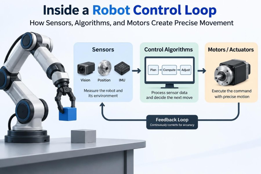
That conversation is the control loop. It connects sensing, computation, and actuation into a repeating process that can happen hundreds or thousands of times each second, depending on the machine and task.
Understanding the loop makes many robotics topics easier to reason about: why an arm shakes, why a mobile robot misses a turn, why tuning can be difficult, and why a powerful motor alone does not make a robot precise.
🔄 The basic idea of feedback control
A closed-loop controller repeatedly compares a desired state with a measured state, calculates a correction, and commands an actuator. The desired state might be a wheel speed, joint angle, room temperature, or drone height.
If a robot arm should move to 45 degrees but its encoder reads 42 degrees, the controller sees an error of 3 degrees. It commands motion in the direction that reduces that error, then measures again. This is called feedback because the outcome feeds back into the next decision.
In an open-loop system, by contrast, a program might simply energize a motor for a fixed time. That can work in highly predictable situations, but it cannot naturally correct for a heavier payload or a slipping wheel.
🎯 Setpoints, states, and error signals
The controller needs a target, often called a setpoint or reference. A target can be a position, velocity, force, orientation, or several quantities at once. The measured quantity is called the process variable or feedback signal.
The simplest error equation is:
error = desired value − measured valueIts sign matters. A positive error tells the controller to correct in one direction; a negative error calls for the opposite direction. In a real robot, engineers also consider units, coordinate frames, sensor offsets, and whether an angle wraps around from 359 degrees to 0 degrees.
👁️ Sensors give the loop its awareness
Sensors convert physical conditions into signals a controller can use. An encoder can report shaft rotation, an inertial measurement unit can estimate angular motion and acceleration, and a force sensor can detect contact at a robot wrist.
A control system is only as useful as the information reaching it. If an encoder misses pulses, a camera has a long delay, or an IMU drifts, the controller can make a logically correct decision from an inaccurate picture of reality.
Good sensor selection starts with the question: what must the robot know to control this task? A line-following robot may need reflected-light measurements; a balancing robot needs body orientation and angular rate.
📏 Position sensing with encoders
Rotary encoders are fundamental in motor control. Incremental encoders produce pulses as a shaft turns, letting software estimate relative position and speed. Absolute encoders report a unique angle after power-up, which can remove the need for a homing move in some designs.
Encoder resolution affects the smallest measurable motion, but high resolution does not automatically create high accuracy. Gear backlash, flexible couplings, mounting misalignment, and wheel slip can separate motor-shaft motion from the motion the robot truly cares about.
For a robot arm, measuring joint rotation is often appropriate. For a wheeled vehicle on loose ground, wheel encoders alone cannot guarantee the vehicle’s location because the wheels may rotate without meaningful travel.
🧭 IMUs and the challenge of moving frames
An IMU typically combines gyroscopes and accelerometers, sometimes with magnetometers. Gyroscopes measure angular rate, while accelerometers sense specific force, which includes the apparent effect of gravity. Together, these signals help a robot estimate how its body is moving.
Raw IMU data is not a ready-made orientation answer. Gyroscope integration accumulates bias over time, and acceleration includes bumps, vibration, and commanded acceleration. Sensor fusion combines complementary measurements to produce a more reliable estimate.
For example, a self-balancing robot needs its tilt angle and tilt rate. Its controller must distinguish a genuine lean from vibration created by the wheels crossing a seam in the floor.
📷 Vision adds context, but also delay
Cameras can recognize objects, estimate pose, read markers, and support navigation. Unlike a motor encoder, however, vision often involves exposure time, image transfer, processing, and detection. That introduces latency: the controller receives information about the recent past.
Vision is therefore often used in a slower, higher-level loop. A camera may locate a part on a conveyor, while a faster encoder-based loop ensures each arm joint follows the commanded trajectory.
Lighting changes, motion blur, occlusion, and calibration errors all affect visual measurements. Treating camera output as certain can create unstable or unsafe behavior, especially around fast motion.
🧹 Filtering noise without hiding the motion
Every measurement contains some uncertainty. Electrical interference, quantization, vibration, and imperfect sensing can make a signal fluctuate. A controller that reacts to every tiny fluctuation may chatter, wear components, and inject noise into the mechanism.
Filters smooth measurements, but they introduce a tradeoff. A stronger low-pass filter reduces high-frequency noise while adding delay. Too much delay can make a fast controller react late and reduce its stability margin.
Useful filtering is tied to the physics of the task. Filter only the frequencies that are unlikely to be meaningful motion, and verify the result using recorded sensor data rather than relying on a visually smooth graph.
🧠 State estimation fills in what cannot be measured directly
Many quantities a robot needs are not measured by one perfect sensor. Velocity may be estimated from successive position readings. A mobile robot’s pose—its position and orientation—may be inferred from wheel encoders, an IMU, and external observations.
This process is called state estimation. It uses a model of expected motion alongside sensor data. A model predicts where the robot should be; measurements pull that prediction back toward observed reality.
Estimates always have limits. If every available sensor is affected by the same failure, or if the model ignores a major physical effect such as wheel slip, combining the signals does not magically make the estimate correct.
🗺️ From a task goal to a motion command
“Pick up the cup” is not a motor command. A robot must convert a task-level goal into a position, orientation, path, and sequence of safe actions. This planning layer decides what motion should occur.
For a mobile robot, a planner may choose a route around obstacles. For an arm, inverse kinematics converts a desired tool pose into candidate joint angles. The control loop then handles the lower-level question: how does each joint reach its assigned target?
Separating planning from control is useful, but the boundary is not rigid. A planner must respect speed, acceleration, workspace, and collision constraints that arise from the physical control problem.
📈 Trajectories prevent abrupt demands
A setpoint is not always a fixed destination. A trajectory specifies how a target changes over time, commonly including position, velocity, and acceleration. It gives the controller a feasible path to follow instead of a sudden step change.
Imagine commanding an arm joint from zero to 90 degrees instantly. The mechanism cannot teleport. A trajectory ramps motion within its torque and speed capabilities, reducing vibration and limiting stress on gears, belts, and payloads.
Trajectory generation matters in additive manufacturing, machining, and pick-and-place work, where smooth movement affects both cycle time and product quality.
⚙️ Actuators turn electrical commands into force
Actuators are the loop’s physical output. Electric motors are common, but robots also use pneumatic cylinders, hydraulic drives, and specialized actuators. A motor controller may regulate current, voltage, torque, speed, or position depending on the system architecture.
Motor torque is closely related to current in many electric motors. This is why sophisticated drives often use an inner current-control loop: it lets the system manage force-producing current quickly before outer loops worry about speed and position.
The actuator is never isolated. Transmission ratios, friction, compliance, payload inertia, and gravity all determine how a motor command becomes actual motion.
🔌 Motor drivers and power electronics
A microcontroller pin cannot directly power a robot arm motor. Motor drivers use power electronics to switch energy from the battery or supply into the motor. For a brushed DC motor, an H-bridge can control direction and apply pulse-width modulation, or PWM, to vary average voltage.
Brushless motors require coordinated switching across multiple phases. Their drivers need rotor-position information from sensors or estimation to produce useful torque efficiently.
Power design affects control behavior. Voltage sag under load, inadequate current capacity, poor grounding, and electrical noise can cause resets or distorted sensor readings that look like mysterious software bugs.
🧮 PID control: the common starting point
The PID controller combines three actions: proportional, integral, and derivative. Its output is often written conceptually as:
output = Kp × error + Ki × accumulated error + Kd × rate of error changeThe proportional term responds to the error now. The integral term accumulates persistent error. The derivative term reacts to how quickly the error is changing. PID is popular because it is understandable, computationally light, and effective for many well-behaved mechanisms.
It is not a universal answer. Systems with severe delay, changing contact conditions, strong nonlinearities, or multiple tightly coupled axes may need additional modeling, feedforward, constraints, or a different control strategy.
📐 What each PID term contributes
| Term | Primary role | Common risk when excessive |
|---|---|---|
| Proportional (P) | Pushes harder when the current error is larger | Oscillation or overshoot |
| Integral (I) | Removes steady bias from friction, gravity, or load | Slow oscillation and windup |
| Derivative (D) | Adds damping by responding to rapid change | Amplifying noisy measurements |
These roles overlap in practice. A well-tuned proportional gain can make a system responsive, but no amount of tuning can overcome a motor that lacks torque for the load or a sensor that reports late.
Derivative action is frequently applied to a measured velocity rather than a numerically differentiated noisy position signal. The exact implementation should match the available sensors and the controller’s sample timing.
🪢 Integral windup and its cure
Integral action is valuable when a robot must hold position against gravity or overcome static friction. But if the actuator saturates—because it has reached its voltage, current, or torque limit—the integral term can keep accumulating error even though the robot cannot respond further.
When the robot finally moves, that stored integral command may drive it past the target. This behavior is known as integral windup.
Common anti-windup methods include limiting the integral state, pausing integration during saturation, or feeding the difference between requested and achievable output back into the integrator. The best choice depends on the controller structure.
⏱️ Sampling time and control-loop rate
Digital controllers act at discrete intervals. Each iteration reads sensors, estimates state, computes a command, and updates outputs. The time between iterations is the sample period; its inverse is the control-loop frequency.
A loop must run fast enough to observe and respond to the system’s meaningful dynamics. A slow thermal process can tolerate leisurely updates. A balancing robot or high-speed motor drive requires much faster and more consistent timing.
Consistency matters as much as average speed. Timing jitter changes the effective behavior of derivative and integral calculations. Use timers, real-time scheduling where appropriate, and measured timestamps rather than assuming every software loop takes exactly the same time.
🏗️ Cascaded loops divide a difficult job
Many robots use nested, or cascaded, loops. An inner loop regulates a fast quantity such as motor current. Around it, a velocity loop commands the required torque. An outer position loop commands the desired velocity.
Each loop has a different job and bandwidth. The inner loop must settle faster than the outer loop so that the outer controller can reasonably treat it as responsive.
This layered arrangement appears in servo drives, drones, and mobile robots. It improves organization and performance, but poor tuning between layers can still create oscillation or sluggishness.
🧲 Feedforward anticipates known effort
Feedback corrects errors after they appear. Feedforward supplies an anticipated command based on what the robot is about to do. For an arm lifting a known load, gravity compensation can command some holding torque before the arm droops.
Other feedforward terms may account for desired velocity, acceleration, friction, or motor characteristics. They reduce the correction burden on feedback and can improve tracking during rapid trajectories.
Feedforward depends on a model, so it is never perfect. A changed payload or worn mechanism can make the estimate wrong. Feedback remains necessary to correct the residual error and unexpected disturbances.
🌪️ Disturbances are part of normal operation
A disturbance is any influence that moves the system away from its intended behavior. A robot vacuum crossing a rug, an arm carrying an unexpectedly heavy item, and a drone meeting wind are all disturbances.
Control performance should be assessed by how the machine responds: how far it deviates, how quickly it recovers, whether it overshoots, and whether it remains stable. A controller that tracks a simple bench test well may struggle once realistic disturbances arrive.
Testing should deliberately include representative loads, directions of travel, battery states, surfaces, and temperatures. This reveals limitations earlier than a single no-load demonstration.
📉 Stability, overshoot, and settling
A stable control loop returns toward its target after a small disturbance. An unstable loop amplifies deviations, potentially producing growing oscillation, violent motion, or repeated saturation.
Engineers describe response using ideas such as rise time, overshoot, steady-state error, and settling time. No single number is always best. A delicate gripper may prioritize low overshoot, while a racing robot may accept some overshoot to turn aggressively.
Stability margins provide room for uncertainty in load, delay, friction, and sensor behavior. A design that is barely stable in a clean simulation may be unreliable when transferred to hardware.
🦿 Mechanical reality changes the controller’s job
Control code cannot erase mechanical problems. Backlash creates a dead zone when a gear train reverses direction. Flexible arms can vibrate. Belt tension changes. Stiction—the tendency to stick before sliding—can make fine motion jerky.
Reducing compliance, improving bearings, choosing suitable gear ratios, routing cables carefully, and placing sensors near the controlled output can simplify control dramatically. Sometimes a mechanical redesign is more effective than increasingly elaborate software.
This is especially relevant when a motor encoder sits before a gearbox. It may report accurate motor position while the end effector moves differently because the transmission flexes or has play.
🧩 Coupled axes require coordinated thinking
In a multi-joint arm, moving one joint can change the forces felt by another. On a quadrotor, each rotor contributes to thrust and body rotation. These are examples of coupled dynamics.
Independent single-axis controllers are often a practical starting point, especially when coupling is mild. As speed, payload, or precision demands increase, engineers may add compensation terms or use controllers that explicitly model interactions.
Coordinate systems also matter. A command expressed in the robot’s tool frame is not automatically the same as one expressed in the base frame. Clear frame definitions prevent subtle, direction-dependent errors.
🧪 A practical tuning workflow
Tuning should be systematic and safety-conscious. Start with conservative output limits and a mechanism that cannot damage itself, nearby people, or test equipment if it moves unexpectedly.
- Verify sensor direction, units, offsets, and realistic readings.
- Verify motor direction and establish output limits.
- Begin with proportional action and observe response to modest commands.
- Add damping or derivative action if the mechanism is underdamped and sensor quality supports it.
- Add only enough integral action to address persistent bias.
- Test trajectories and disturbances, not merely a stationary setpoint.
Record commands, measurements, errors, and saturation flags. A time plot is far more revealing than tuning by intuition alone.
🛑 Saturation and safety limits are control features
Every actuator has limits. A controller may request more voltage, torque, or speed than the hardware can provide. Explicit saturation limits keep commands inside electrical and mechanical boundaries, but they also change the controller’s response.
Robots need separate safety measures beyond ordinary control logic: emergency stops, travel limits, current limits, watchdogs, fault detection, and safe startup behavior. A stable algorithm cannot protect against every wiring fault, software crash, or failed sensor.
For collaborative or high-energy equipment, safety design must be based on the machine, environment, applicable requirements, and professional risk assessment—not on software confidence alone.
🔍 Logging turns symptoms into evidence
When a robot “acts weird,” log the loop. At minimum, capture time, setpoint, measured state, controller output, and saturation state. For complex systems, include estimates, mode changes, battery voltage, fault flags, and relevant sensor health data.
A plot can distinguish several similar-looking problems. A delayed measurement may cause phase lag; insufficient torque may show sustained saturation; encoder noise may appear as a jagged derivative signal; a sign error can make error grow immediately.
Logging also supports repeatable comparisons after a code or hardware change. Without it, teams can easily mistake a different battery charge or floor surface for an improvement in control design.
🐛 Common implementation mistakes
- Wrong sign conventions: positive error produces motion that increases the error.
- Mixed units: degrees, radians, encoder counts, and meters are combined without explicit conversion.
- Ignoring elapsed time: integral and derivative calculations assume a fixed interval that software does not maintain.
- Unfiltered derivative noise: measurement noise becomes aggressive motor commands.
- No saturation handling: the integrator accumulates impossible commands.
- Testing only one condition: a tuned controller fails when direction, payload, or supply voltage changes.
These failures are mundane, which is exactly why disciplined interfaces, unit tests, calibration routines, and data logs are so valuable.
🚗 Example: holding speed on a mobile robot
Consider a two-wheeled robot commanded to travel at a steady speed. Wheel encoders measure rotation, software estimates each wheel’s speed, and a velocity controller adjusts motor commands to reduce the difference from the target.
When the robot reaches carpet, the required torque rises. An open-loop command may let it slow down. A closed-loop velocity controller notices the measured speed drop and requests more motor effort, up to its allowed limit.
This does not guarantee straight travel. Uneven traction or motor mismatch can make one wheel behave differently. An outer heading loop, using an IMU or other heading estimate, can adjust left and right wheel targets to keep the chassis aligned.
🤏 Example: a gripper making gentle contact
Position control is ideal until a gripper touches a fragile object. After contact, continuing to force a position setpoint can apply excessive force because the object blocks the commanded motion.
A compliant gripper may switch to force control, torque limiting, or impedance control. Impedance control shapes how the robot responds to displacement, making it behave more like a chosen spring-damper system rather than a perfectly rigid position source.
Contact tasks highlight a central control lesson: the right controlled variable changes with the task. Precision does not always mean refusing to yield; sometimes it means applying a carefully limited force.
🧰 Choosing the right level of complexity
A simple PID loop with an encoder can be excellent for a conveyor, small servo, or educational mobile robot. It is easier to inspect, tune, and maintain than a more elaborate design.
More advanced methods become worthwhile when constraints, coupling, changing dynamics, or safety-critical tracking demand them. Examples include model-based control, adaptive approaches, optimization-based methods, and robust control techniques.
Complexity should solve a demonstrated problem. Before replacing a basic controller, check sensor quality, timing, saturation, mechanics, trajectory design, and calibration. Many apparent “algorithm problems” begin elsewhere.
🔗 The core principle: measure, decide, act, repeat
Precise robot movement is not produced by a single component. Sensors reveal the current state, estimation interprets imperfect measurements, planning defines feasible goals, algorithms compute corrections, and actuators apply force to the physical world.
Each part affects the others. Better mechanics can reduce the control burden; better timing can improve stability; a sensible trajectory can prevent actuator saturation; and useful logs can turn trial-and-error into engineering evidence.
The loop succeeds when its model of the robot stays close enough to reality, its corrections arrive soon enough, and its commands remain within what the mechanism can safely deliver.
A robot moves precisely not because it never makes an error, but because it detects error quickly and corrects it intelligently, again and again. That is the practical power of closed-loop control. 🦾🔄📐