
Robots are expected to move with remarkable precision. A robotic arm assembling electronics may need to place a component within fractions of a millimeter, an autonomous vehicle must maintain a desired steering angle, and a camera gimbal must remain steady even when the platform beneath it is moving.
Achieving this level of accuracy requires more than simply commanding a motor to turn for a certain amount of time.
Motors encounter changing loads, friction, mechanical backlash, gravity, vibration, battery-voltage variations, and external disturbances. If a controller merely tells a motor to move without continuously checking the result, the robot may stop too early, overshoot its target, or drift away from the desired position.
One of the most widely used solutions is PID control. ⚙️🎯
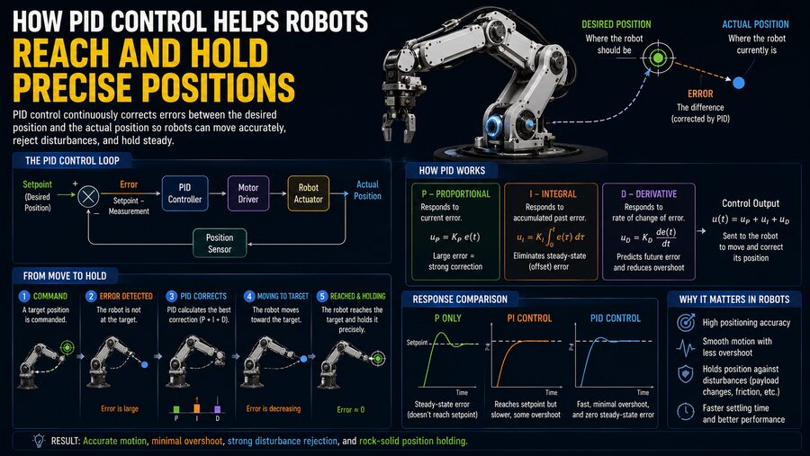
PID stands for Proportional, Integral, and Derivative. A PID controller continuously compares the robot’s desired position with its actual measured position. It calculates the difference—called the error—and adjusts the motor command in an attempt to reduce that error.
This feedback process can happen hundreds or thousands of times per second, enabling robots to reach targets smoothly and hold their positions even when conditions change.
🎯 The Basic Position-Control Problem
Suppose a robotic joint is currently positioned at:
30°
The control system wants it to move to:
75°
The desired position is called the setpoint.
A sensor such as an encoder measures the actual position.
The controller calculates:
Error = Desired Position − Actual Position
So initially:
Error = 75° − 30° = 45°
Because the error is large, the controller commands the motor to produce significant motion toward 75°.
As the joint approaches its destination, the error becomes smaller.
At 70°:
Error = 75° − 70° = 5°
The controller therefore reduces its output.
Eventually, the joint reaches approximately 75° and the error approaches zero.
This process is known as closed-loop feedback control.
🔄 Open-Loop vs. Closed-Loop Control
To understand PID, it helps to compare closed-loop control with open-loop control.
An open-loop system sends a command without measuring whether the desired result was actually achieved.
For example:
Run motor at 50% power for two seconds.
This assumes that two seconds of operation will always produce the same movement.
In reality, the robot might be carrying a heavier load than usual. Friction could increase. The battery voltage could fall. The motor might therefore travel a different distance.
A closed-loop controller instead measures the result:
Command → Motor moves → Sensor measures position → Controller checks error → Command is corrected
This continuous feedback allows the system to compensate for real-world uncertainty.
🧠 What Does PID Mean?
A PID controller combines three different responses:
- P — Proportional
- I — Integral
- D — Derivative
Its control output is often expressed as:
u(t) = Kp·e(t) + Ki∫e(t)dt + Kd·de(t)/dt
where:
- u(t) = controller output
- e(t) = position error
- Kp = proportional gain
- Ki = integral gain
- Kd = derivative gain
Each term contributes differently to robot behavior.
Together, they can produce fast, accurate, and stable positioning.
⚡ The Proportional Term
The proportional term responds directly to the current error.
It can be written as:
P = Kp × Error
If the robot is far from its target, the proportional response is large.
If it is close to the target, the response becomes smaller.
Imagine a robot joint that is 20° away from its desired position.
A strong proportional controller commands substantial torque.
When the joint is only 2° away, the command becomes much smaller.
This makes intuitive sense:
Large error → Strong correction
Small error → Gentle correction
The proportional term is often the main driver of movement toward the target.
🚀 What Happens If Proportional Gain Is Too Low?
If Kp is too small, the robot responds weakly.
Possible symptoms include:
- Slow movement
- Sluggish correction
- Poor resistance to disturbances
- Failure to reach the target accurately
A robotic arm may approach its position very slowly or stop slightly short because the remaining error produces too little motor torque to overcome friction or gravity.
⚠️ What Happens If Proportional Gain Is Too High?
Increasing Kp makes the controller more aggressive.
At first, this improves response speed.
But if Kp becomes too large, the robot may repeatedly overshoot the target.
For example:
Target = 90°
The joint reaches:
94° → 87° → 92° → 89° → 91°
The system oscillates around the target.
Extremely high proportional gain can even make the system unstable.
This illustrates an important control-engineering principle:
Faster response is not always better if stability is lost.
🧮 The Integral Term
The integral term looks at accumulated error over time.
Conceptually:
I = Ki × Accumulated Error
Suppose a robotic joint should hold at 45°, but gravity continually pulls it downward.
The proportional controller may settle at 44.5° because a small remaining error is necessary to produce enough motor torque to oppose gravity.
This is called steady-state error.
The integral term solves this problem by remembering that the error has persisted.
If the robot remains 0.5° below the target, that error accumulates over time.
The integral contribution gradually increases until enough additional motor command is produced to eliminate the remaining error.
This allows the robot to settle much closer to the exact setpoint. 🎯
🏋️ Integral Control Helps Fight Constant Loads
Integral action is especially useful when a robot must resist persistent disturbances.
Examples include:
- Gravity pulling on a robotic arm
- Constant friction
- Conveyor belt resistance
- Uneven mechanical loading
- Persistent external force
Without integral action, the controller may accept a small offset.
With integral action, even a tiny persistent error continues to build correction until the offset is removed.
⚠️ Integral Windup
Integral control introduces a potential problem called integral windup.
Imagine a robot is commanded to move far beyond its current position.
The motor reaches its maximum possible output, but the error remains large.
The integral term continues accumulating error even though the actuator cannot produce more torque.
Eventually, the robot approaches the target—but the accumulated integral value is now enormous.
The controller may continue commanding excessive motion, causing large overshoot.
This is integral windup.
Engineers prevent it using anti-windup techniques such as:
- Limiting the integral value
- Stopping integration during actuator saturation
- Resetting the integral term under certain conditions
- Feeding saturation information back into the controller
Anti-windup is especially important in robotic systems where motors have strict torque and voltage limits.
🛑 The Derivative Term
The derivative term responds to how quickly the error is changing.
Conceptually:
D = Kd × Rate of Change of Error
If a robot is rapidly approaching its target, the derivative term detects that the error is shrinking quickly.
It can then reduce the motor command before the robot reaches the target.
This acts somewhat like damping or predictive braking. 🛑
Consider driving a car toward a stop sign.
The proportional term is like knowing how far away the stop sign is.
The derivative term is like knowing how quickly you are approaching it.
If you are moving rapidly toward the target, you need to start braking sooner.
🎢 How Derivative Control Reduces Overshoot
Without sufficient damping, a robot joint may carry momentum past its target.
The derivative term opposes rapid changes and can reduce this overshoot.
It helps produce:
- Smoother stopping
- Reduced oscillation
- Better stability
- Faster settling
This is especially useful in systems with noticeable inertia.
Robotic arms, camera platforms, and mobile robots all contain mechanical mass that cannot stop instantaneously.
📡 Derivative Control and Sensor Noise
Derivative control also has an important weakness.
Because it responds to rapid changes, it can amplify measurement noise.
Suppose an encoder reading fluctuates slightly:
50.00° → 50.03° → 49.98° → 50.02°
These changes are tiny, but they occur quickly.
A derivative term may interpret them as significant motion and produce a noisy control signal.
Engineers often reduce this problem using:
- Low-pass filtering
- Filtered derivative terms
- High-quality sensors
- Appropriate sampling rates
Many practical PID controllers therefore use a derivative calculation that is intentionally filtered.
🧩 How the Three PID Terms Work Together
The three terms complement one another.
⚡ Proportional
Pushes the robot toward the target according to current error.
🧮 Integral
Eliminates persistent position offsets.
🛑 Derivative
Damps the response and anticipates overshoot.
A useful conceptual summary is:
P reacts to the present.
I remembers the past.
D anticipates the near future based on current motion.
This combination allows a well-tuned robot to move rapidly without excessive overshoot and settle accurately at the desired position.
🦾 Example: Robotic Arm Joint
Consider a robotic arm lifting an object.
The target joint angle is:
60°
The actual joint angle begins at:
20°
Initially, the position error is 40°.
The proportional term produces strong motor torque.
As the arm moves upward, the error decreases.
Because the arm has inertia, the derivative term begins reducing the command as it approaches 60°.
Gravity may cause the arm to settle slightly below the target.
The integral term detects the persistent error and gradually increases motor torque.
Eventually:
Measured position ≈ 60°
If someone places additional weight on the arm, the joint may sag.
The controller immediately detects the new error and increases torque to restore the commanded position.
This is why feedback control is so powerful.
🔢 Encoders Provide Position Feedback
PID position control depends on accurate measurement.
Robots commonly use encoders to measure joint or motor position.
Encoders may be:
- Optical
- Magnetic
- Incremental
- Absolute
An incremental encoder generates pulses as the shaft rotates.
The controller counts these pulses to estimate position.
An absolute encoder provides a unique code representing its shaft angle.
Without reliable position feedback, the PID controller does not know whether the robot has actually reached its target.
⚙️ Motor Drivers Convert PID Output Into Motion
The PID controller does not usually power the motor directly.
Instead, it calculates a requested control output.
This output may represent:
- Voltage
- Current
- Torque
- PWM duty cycle
A motor driver or power inverter then converts this command into electrical power for the motor.
A simplified control loop is:
Target position → PID controller → Motor driver → Motor → Robot joint → Encoder → PID controller
This loop repeats continuously.
⏱️ Why Control-Loop Frequency Matters
PID calculations are performed at regular intervals.
A small hobby robot might update its controller hundreds of times per second.
High-performance robotic systems may use control loops operating at kilohertz rates.
If updates are too slow, the controller reacts late.
A robot may overshoot or become unstable.
If updates are extremely fast, computation and sensor noise can become more important.
The selected control frequency must be appropriate for the mechanical dynamics of the robot.
🎚️ PID Tuning
Choosing the values of Kp, Ki, and Kd is called PID tuning.
Poorly tuned gains can make even high-quality hardware perform badly.
A controller with inadequate tuning may be:
- Too slow
- Too aggressive
- Oscillatory
- Noisy
- Unable to hold position
The objective is generally to achieve a desirable balance between:
- Rise time
- Overshoot
- Settling time
- Steady-state error
- Robustness
There is no universal set of PID gains that works for every robot.
🔧 Manual PID Tuning
One common practical method begins by setting integral and derivative gains relatively low or to zero.
The engineer increases proportional gain until the system responds strongly but remains manageable.
Derivative action is then introduced to reduce oscillation and overshoot.
Finally, a modest integral term may be added to eliminate persistent steady-state error.
The procedure varies with the system, and safety limits should always be applied during testing.
Large industrial robots require controlled commissioning procedures rather than aggressive trial-and-error tuning.
📊 Ziegler-Nichols and Other Tuning Methods
Formal PID tuning approaches also exist.
One historically important family of methods is Ziegler-Nichols tuning.
Other approaches include:
- Model-based tuning
- Relay auto-tuning
- Optimization-based tuning
- Frequency-response methods
Modern industrial controllers may include automatic tuning functions.
However, automated methods still require engineers to verify the resulting behavior.
A mathematically responsive controller may not be appropriate if it causes excessive mechanical stress.
📈 Rise Time
Rise time describes how quickly the robot approaches its target after receiving a command.
A low proportional gain may produce a long rise time.
Increasing the gain usually improves response speed—up to the point where overshoot and instability become concerns.
Fast-moving robots often require carefully optimized rise time.
🎯 Overshoot
Overshoot occurs when the robot passes beyond its desired position.
For example:
Commanded position = 100 mm
Maximum actual position = 108 mm
The robot has overshot by 8 mm.
Small overshoot may be acceptable in some systems.
In precision manufacturing, overshoot could cause collisions or damage.
Derivative action and trajectory planning can help reduce it.
⏳ Settling Time
Even after reaching the target, a robot may oscillate around it.
Settling time describes how long the system takes to remain within an acceptable tolerance around the setpoint.
For example, engineers might define the position as settled when it remains within:
±0.1°
A good controller often aims for both fast movement and short settling time.
🎯 Steady-State Error
Steady-state error is the remaining difference between desired and actual position after transient motion has ended.
A proportional-only controller may leave a persistent offset.
Integral control is commonly used to reduce or eliminate it.
For high-precision robotics, even tiny steady-state errors can matter.
🏭 PID in Industrial Robots
Industrial robotic arms often perform repetitive operations such as:
- Welding
- Painting
- Assembly
- Packaging
- Material handling
Each joint contains a servo motor and feedback sensors.
Controllers continuously regulate position, velocity, and torque.
Real industrial servo systems may use more sophisticated methods than a single PID loop, but PID-based control remains an important foundation.
🔄 Cascaded PID Loops
High-performance motor control often uses cascaded control loops.
Instead of one controller directly controlling everything, several loops operate inside one another.
A common structure is:
Position loop → Velocity loop → Current/Torque loop
The outer position controller determines how fast the motor should move.
The velocity controller determines how much torque is needed.
The current controller regulates motor current.
The inner loops operate faster than the outer loops.
This layered structure provides excellent control of robotic actuators.
⚡ Current Control and Torque
For many electric motors, torque is closely related to electrical current.
This makes current control extremely useful.
The innermost servo loop can regulate current very rapidly.
The position PID then indirectly controls torque through the velocity and current loops.
This gives robots precise motion while protecting motors and power electronics from excessive current.
🧭 PID for Mobile Robot Steering
PID control is also useful in mobile robots.
Suppose an autonomous robot must maintain a heading of:
90°
Sensors indicate the current heading is:
85°
The controller detects a 5° error and adjusts wheel speeds or steering.
As the robot turns toward 90°, the correction decreases.
If wind, uneven terrain, or wheel slip pushes it away from the desired heading, the PID controller responds automatically.
This same principle can help control:
- Heading
- Speed
- Path tracking
- Wheel position
🚁 PID in Drones
Multirotor drones are famous examples of feedback control.
A drone must continuously stabilize:
- Roll
- Pitch
- Yaw
- Altitude
Tiny disturbances from wind can cause rapid movement.
Sensors such as gyroscopes and accelerometers measure the drone’s orientation and motion.
PID-style controllers adjust motor speeds many times per second.
Without active feedback, a multirotor drone would be extremely difficult to keep stable. 🚁
📷 Camera Gimbals
Camera gimbals use precise feedback control to keep cameras steady.
When the platform rotates, sensors detect the motion.
The controller commands motors to rotate the camera in the opposite direction.
PID control can help remove:
- Hand shake
- Vehicle vibration
- Drone movement
Smooth derivative damping is especially useful because visible oscillation would make the recorded video unstable.
🏭 CNC Machines and Precision Positioning
Computer numerical control machines require extremely accurate axis positioning.
Servo motors move cutting tools or workpieces along controlled paths.
Feedback systems continually compare commanded and measured position.
Errors may be only micrometers.
While advanced motion-control systems incorporate feedforward and trajectory algorithms, PID-style feedback remains a central concept.
🧲 Holding Position Against Disturbances
Reaching a target is only half the problem.
A robot often needs to hold that target.
Suppose a robot arm is holding a tool at a fixed angle.
An external force pushes the tool downward.
The encoder immediately detects a position change.
The PID controller increases motor torque and returns the arm toward the desired position.
The control loop continuously repeats this correction.
This makes the robot behave as though it has an electronic restoring force.
🌍 Gravity Compensation
Robotic arms are constantly affected by gravity.
A joint supporting a horizontal arm may require significant torque even when completely stationary.
PID control can compensate for this, but engineers often improve performance using gravity compensation.
A mathematical model predicts the torque required to support the arm.
That torque is applied as a feedforward command.
The PID controller then handles only the remaining errors.
This reduces the burden on the integral term and improves responsiveness.
⏩ Feedforward Plus PID
Feedforward control predicts the actuator command required before error appears.
For example, if a robot model predicts that 4 Nm of torque is needed to support a link, the controller can command approximately 4 Nm immediately.
PID feedback then corrects imperfections in the model.
A common architecture is therefore:
Control Output = Feedforward + PID Correction
This combination is extremely powerful in robotics.
🛤️ Trajectory Tracking
Robots rarely jump instantly from one position command to another.
Instead, motion planners create smooth trajectories describing how position should change over time.
A trajectory may specify:
- Position
- Velocity
- Acceleration
The PID controller attempts to keep the real mechanism close to that trajectory.
This avoids sudden motor commands and reduces mechanical stress.
Smooth trajectory planning is especially important for large robotic arms and high-speed machinery.
⚠️ Actuator Saturation
Motors have physical limits.
A controller may request more torque or speed than the actuator can deliver.
This condition is called saturation.
For example:
Requested motor voltage = 30 V
but:
Available supply = 24 V
The driver cannot provide the requested output.
PID designs therefore include output limits.
Integral anti-windup is particularly important whenever saturation occurs.
⚙️ Friction and Backlash
Mechanical imperfections make position control more difficult.
Friction can prevent small controller outputs from moving the mechanism.
Backlash creates a small range in which motor motion does not immediately translate into joint motion.
These effects can cause:
- Position errors
- Oscillation
- Hysteresis
Engineers may compensate using better mechanical design, feedforward models, or specialized nonlinear control techniques.
PID alone cannot remove every physical limitation.
🧠 Why PID Remains Popular
Many advanced control methods exist, including:
- State-space control
- Model predictive control
- Adaptive control
- Robust control
- Nonlinear control
Yet PID remains extremely common.
Why?
Because it is:
- Relatively simple
- Computationally inexpensive
- Well understood
- Easy to implement
- Effective for many systems
- Supported by enormous engineering experience
A microcontroller can execute a PID controller with very little computation.
That makes it suitable for everything from hobby robots to industrial machinery.
🛡️ Safety Limits in Robotic PID Systems
A position controller should never be allowed unlimited authority.
Robotic systems typically include protections such as:
- Maximum motor current
- Maximum torque
- Position limits
- Velocity limits
- Emergency stops
- Collision detection
If a sensor fails and reports an incorrect position, an unrestricted controller might command dangerous motion.
Safety systems therefore operate alongside normal PID control.
🤖 Adaptive and Auto-Tuning Controllers
A fixed set of PID gains may not perform equally well under all conditions.
A robot arm behaves differently when empty compared with when carrying a heavy payload.
Some advanced systems adjust controller parameters according to operating conditions.
This can involve:
- Gain scheduling
- Adaptive control
- Automatic tuning
For example, a controller may use different gains depending on arm configuration or payload weight.
🔬 PID Is Not Perfect for Every Robot
PID works especially well when the controlled system behaves reasonably predictably around its operating range.
Highly nonlinear robots, flexible structures, strong joint coupling, or extreme dynamic motion may require additional techniques.
Advanced controllers can explicitly account for robot dynamics.
Nevertheless, PID is often still used at lower actuator-control levels because of its simplicity and robustness.
🧪 A Simple Discrete PID Implementation
Digital robot controllers calculate PID at discrete time intervals.
A simplified implementation may follow:
error = target_position - measured_position

integral = integral + error × dt

derivative = (error - previous_error) / dt

output = Kp × error
       + Ki × integral
       + Kd × derivative

previous_error = error
This loop repeats continuously.
Real implementations usually add:
- Output saturation
- Integral limits
- Derivative filtering
- Sensor filtering
- Timing checks
These details are important for reliable hardware control.
📊 What a Well-Tuned Response Looks Like
Suppose a robot receives a step command from 0° to 45°.
A well-tuned response might:
- Accelerate rapidly toward 45°.
- Begin slowing before reaching the target.
- Produce little or no overshoot.
- Settle quickly.
- Hold 45° despite disturbances.
Poor tuning might instead produce:
Slow response → Large overshoot → Repeated oscillation → Long settling time
Control engineers examine plots of position versus time to evaluate these characteristics.
🔋 Efficiency Benefits
Accurate control can also improve energy efficiency.
An unstable controller that continuously oscillates forces the motor to accelerate and decelerate unnecessarily.
This consumes power and creates heat.
A well-tuned controller minimizes unnecessary correction while still maintaining accuracy.
For battery-powered robots, these savings can contribute to longer operating time.
🌐 PID in Collaborative Robots
Collaborative robots, or cobots, operate near people.
Their controllers must provide precise position regulation while also respecting force and speed limits.
PID-based servo loops may form part of the low-level actuator control.
Higher-level safety and force-control systems monitor the robot to ensure safe interaction.
Precise feedback control enables these machines to move smoothly and predictably.
🧠 The Bigger Control-System Picture
PID should not be viewed as an isolated formula.
In a real robot, precise positioning depends on the entire system:
Motion planner → Desired trajectory → PID/servo controller → Motor driver → Motor and gearbox → Robot mechanism → Encoder → Feedback
Performance is affected by every component.
A perfect PID controller cannot compensate for an extremely inaccurate sensor or badly damaged gearbox.
Similarly, excellent motors cannot provide precise motion without good feedback and control.
Robotic precision is therefore a system-level achievement.
✨ Conclusion
PID control helps robots reach and hold precise positions by continuously measuring the difference between a desired position and the robot’s actual position.
The proportional term reacts to current error and provides the main force driving the robot toward its target.
The integral term accumulates persistent error and helps eliminate small position offsets caused by effects such as gravity and friction.
The derivative term observes how quickly error is changing and provides damping that can reduce overshoot and oscillation. ⚙️🎯
Combined with encoders, motor drivers, high-speed digital controllers, and carefully selected gains, PID can make a robotic joint move quickly toward its destination, slow smoothly as it approaches, and continuously resist disturbances once it arrives.
Real robotic systems often extend the concept with cascaded position, velocity, and current loops; feedforward control; gravity compensation; trajectory planning; anti-windup; and safety limits.
Yet the fundamental idea remains simple:
Measure the error → Calculate a correction → Move the robot → Measure again.
This loop may execute thousands of times every second.
That continuous cycle is what allows a mechanical system affected by friction, inertia, changing loads, and external forces to behave with remarkable accuracy. 🤖⚡
From industrial robot arms and CNC machines to drones, autonomous vehicles, and camera gimbals, PID control remains one of the foundational tools that turns electric motors into precise, responsive robotic motion.