
A robot arm reaches for a coffee mug, a warehouse robot lowers a package onto a conveyor, and a surgical tool changes angle inside a small working area. In each case, the task sounds simple: move the tool to the right place.
But a robot cannot begin with the human instruction “put your hand there.” Its motors do not directly control a point in space. They rotate joints, slide rails, or extend actuators, each with its own range, speed, and physical constraints.
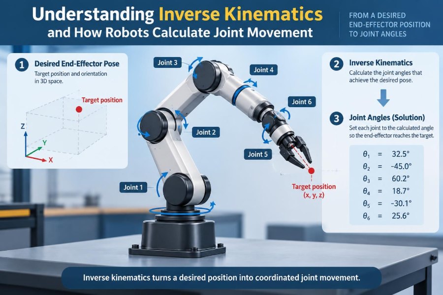
The calculation that translates a desired tool position into joint movements is called inverse kinematics, usually shortened to IK. It is one of the central ideas that turns a mechanical structure into a useful, coordinated machine.
Understanding IK helps students connect geometry, programming, and control. For working engineers, it clarifies why a robot can reach one target smoothly, struggle with another, or report that a perfectly reasonable-looking pose is impossible.
🧭 From a Goal in Space to Motor Commands
Inverse kinematics starts with a desired pose: the position and orientation of a robot’s end effector. The end effector may be a gripper, welding torch, camera, suction cup, or any tool mounted at the end of a mechanism.
The IK problem asks: which values should every joint take so that this tool reaches that pose? Those values are then passed to motion-planning and motor-control systems, which determine a safe trajectory and drive the hardware.
🔄 Forward Kinematics Comes First
Before solving inverse kinematics, engineers define forward kinematics. Forward kinematics takes known joint values and calculates where the end effector will be.
For example, if a two-link arm’s shoulder rotates 30 degrees and elbow rotates 45 degrees, geometry can calculate the gripper’s coordinates. IK reverses that direction: given coordinates, find suitable shoulder and elbow angles.
Forward kinematics is generally direct. Inverse kinematics can have multiple answers, no answer, or answers that are technically correct but undesirable.
🦿 Joints Are the Robot’s Degrees of Freedom
A robot’s degrees of freedom, or DOF, are its independently controllable motions. A rotating joint contributes one rotational DOF; a linear slide contributes one translational DOF.
A common industrial manipulator has six joints because positioning a rigid tool freely in three-dimensional space usually involves three position components and three orientation components. More joints can add flexibility, while fewer joints limit the poses the robot can achieve.
📍 Position and Orientation Are Different Targets
Reaching a point is not always enough. A suction gripper may only need to arrive above a box, but a welding torch must hold a particular angle, and a screwdriver must align with a screw axis.
Position is often represented by Cartesian coordinates (x, y, z). Orientation describes how the tool is rotated. Engineers may represent orientation with rotation matrices, Euler angles, or quaternions; each representation has practical advantages and pitfalls.
📐 Coordinate Frames Keep Geometry Consistent
Robotic calculations use named coordinate frames: a base frame fixed to the robot, a frame for each link, a tool frame at the end effector, and often a workpiece or camera frame.
A target reported by a vision system may be expressed relative to the camera. To use it, software transforms that target through calibrated frame relationships into the robot base frame. A correct IK solver cannot compensate for incorrect frame definitions.
🧱 Links, Offsets, and the Kinematic Chain
A kinematic chain is the ordered sequence of rigid links and joints between the robot base and its tool. Each joint changes the pose of everything downstream from it.
Even a visually simple arm includes details that matter: link lengths, joint-axis directions, fixed offsets, and tool mounting distance. Small modeling errors can create noticeable positioning errors at the tool tip because errors accumulate along the chain.
✏️ A Two-Link Arm Makes IK Visible
Consider a hypothetical planar arm with two links of lengths L1 and L2. Its shoulder angle is q1, elbow angle is q2, and its gripper target is (x, y).
The target’s distance from the shoulder is r = √(x² + y²). If r is longer than L1 + L2, the target lies beyond the arm’s maximum reach. If it is too close for the folded geometry, it can also be unreachable.
For reachable points, the law of cosines provides an elbow-angle relationship. The shoulder angle then follows from the target direction and the geometry of the triangle. This simple example contains many of the same decisions found in larger robots.
🪞 One Target Can Have Several Solutions
A two-link arm can often reach the same point with an “elbow-up” or “elbow-down” posture. Both satisfy the endpoint geometry, but they place the links differently in the workspace.
Six-axis robots can have several discrete joint configurations for one tool pose. The controller needs a rule for choosing among them, such as staying near the current posture, avoiding obstacles, or maintaining clearance from a fixture.
🚫 Some Targets Have No Valid Solution
A target may be unreachable because it is outside the robot’s geometric workspace. It may also be geometrically reachable but invalid because a joint limit, collision constraint, cable restriction, or tool orientation requirement rules it out.
That distinction matters in debugging. “No IK solution” does not always mean the arm is too short; it can mean the requested orientation forces an impossible wrist posture.
🗺️ Workspace Is More Than a Reach Radius
A robot’s workspace is the set of poses it can attain, not merely a sphere or circle around its base. Obstacles, joint limits, and required orientations can carve large gaps out of the apparent reach volume.
When designing a cell, engineers check the reachable workspace with the actual tool attached. A long gripper changes both the reachable area and the risk of striking nearby equipment.
🔒 Joint Limits Make Solutions Realistic
Physical joints cannot rotate forever. Limits protect mechanical stops, hoses, wiring, gears, and people working near the machine. An IK solution outside a limit is not useful, even if the equations produce it.
Good solvers either enforce limits during the search or reject invalid candidates afterward. In applications with tight access, limit-aware solving prevents a system from repeatedly selecting a mathematically neat but physically impossible posture.
⚖️ Redundancy Adds Choice—and Complexity
A robot is redundant when it has more controllable DOF than the task strictly requires. A seven-joint arm, for example, can often hold the same tool pose while changing its elbow position.
This extra freedom is valuable for avoiding obstacles, preserving dexterity, or keeping a camera view open. Yet it also means IK has infinitely many potential solutions, so engineers must define secondary goals rather than expect a single natural answer.
🧮 Closed-Form IK Uses Derived Equations
For certain robot geometries, engineers can derive an analytic, or closed-form, IK solution. The solver applies trigonometry and algebra to calculate each allowable joint configuration directly.
Analytic IK is fast and can enumerate configurations reliably when the mechanism matches the derivation. Its drawback is specificity: a small geometry change, an unusual joint layout, or added redundancy can make the derivation difficult or impractical.
🔢 Numerical IK Searches for an Answer
Numerical IK begins with a guessed joint configuration, computes the current tool pose, measures the error from the target, and iteratively adjusts joints to reduce that error.
This approach is flexible and works with complex kinematic chains. However, it depends on settings such as the initial guess, step size, stopping tolerance, iteration limit, and treatment of constraints.
📊 The Jacobian Connects Joint Motion to Tool Motion
The Jacobian is a matrix that locally relates small joint changes to small end-effector changes. In compact form, it maps joint velocity to tool velocity.
Numerical solvers use the Jacobian to estimate which joint changes will reduce position and orientation error. It is a local model, so a large move is usually broken into repeated small updates rather than solved as one uncontrolled correction.
🧩 Error Must Be Measured Carefully
An IK solver compares desired and current pose. Position error has distance units, while orientation error is angular, so combining them requires thoughtful weighting.
If orientation receives too little weight, the tool may reach the right location with the wrong angle. If it receives too much, the solver may sacrifice useful position accuracy while chasing a minor rotational difference. The correct balance depends on the process.
🌀 Singularities Reduce Useful Motion
A singularity occurs where the robot loses one or more instantaneous motion capabilities, or where small tool motions demand very large joint velocities. A fully stretched arm is a familiar simple example.
Near a singularity, numerical calculations can become unstable and motors may need abrupt motion. Controllers often detect these regions, reduce speed, choose another configuration, or use damping methods that trade exactness for smoother behavior.
🧯 Damped Least Squares Improves Stability
One common numerical technique is damped least squares. Instead of aggressively inverting a poorly conditioned Jacobian near a singularity, the method adds a damping term that limits extreme joint updates.
The trade-off is intentional: the tool may not follow the requested infinitesimal motion perfectly, but the robot avoids unrealistic velocity commands. Damping must be tuned; excessive damping can make a solver slow or inaccurate.
🎯 The Starting Guess Influences Numerical IK
Numerical IK is local. Starting near an elbow-up posture may lead to elbow-up, while starting near elbow-down may converge to a different valid solution.
For continuous robot motion, using the previous successful joint state as the next initial guess usually promotes smooth behavior. Randomly restarting from unrelated configurations can cause posture jumps even when the target changes only slightly.
🛤️ IK Solves Poses, Planning Solves Paths
IK answers whether and how a particular target pose can be achieved. Motion planning answers how to travel from the current joint state to that solution without collisions, limit violations, or unacceptable motion.
Directly interpolating between two valid joint configurations can still sweep the tool through an obstacle. Conversely, a collision-free Cartesian path may require solving IK at many intermediate waypoints.
🧱 Collision Checking Cannot Be an Afterthought
Robot links, tools, fixtures, floor stands, and nearby robots all occupy space. A posture that places the tool safely at its target may still put an elbow through a machine guard.
Practical systems use geometric collision models during planning and, where appropriate, during IK selection. Accurate models matter, but so do conservative safety margins that account for calibration error, payload deflection, and uncertainty.
📦 Payload Changes the Physical Outcome
Kinematics describes geometry, not force. A joint configuration can be valid in IK yet perform poorly when a heavy payload causes flex, torque saturation, vibration, or slower acceleration.
This is why industrial applications pair IK with dynamics, load data, speed limits, and controller monitoring. A pose that is acceptable for an empty gripper may not be suitable for a loaded tool at high speed.
👁️ Vision-Guided Robots Need Calibration
In vision-guided picking, a camera detects an object and reports its location. IK only becomes useful after the system knows the camera-to-robot transformation and the tool’s actual pickup point.
Hand-eye calibration estimates these relationships. If the camera frame, robot base frame, or tool center point is wrong, the IK solution may be internally correct while the gripper consistently misses the real object.
🛠️ The Tool Center Point Defines the Real Target
The tool center point (TCP) is the reference point on the end effector that the robot treats as its operational tip. For a welder, it may be the electrode tip; for a gripper, it may be the center between fingers.
Changing tools without updating the TCP shifts every commanded pose. A few centimeters of unmodeled tool extension can turn a good offline program into a collision or a failed pick.
🧪 Simulation Helps, but Hardware Has the Final Say
Simulation is excellent for visualizing reachability, configurations, and planned motion before equipment moves. It can reveal a poor layout or singular posture early, when changes are cheaper.
But simulation depends on its model. Real robots have backlash, compliance, sensor noise, calibration drift, controller-specific behavior, and imperfectly known environments. Validate slowly on hardware with appropriate safeguards.
⚠️ Common IK Implementation Mistakes
- Mixing units: combining degrees in one component and radians in another produces plausible-looking but wrong motion.
- Ignoring frame conventions: an axis sign or transform order error can mirror or offset the result.
- Accepting convergence blindly: a low numerical error does not prove the solution is collision-free or within limits.
- Forgetting angle wraparound: rotations near equivalent values can appear far apart unless handled consistently.
- Commanding discontinuous solutions: switching branches without checking joint distance can create sudden motion.
✅ A Practical IK Workflow
- Define the robot, joint axes, link dimensions, joint limits, and TCP accurately.
- Establish consistent coordinate frames and verify forward kinematics against known poses.
- Specify the target pose and task tolerances for position and orientation.
- Generate analytic candidates or run a numerical solver from a sensible seed.
- Reject solutions that violate limits, collisions, singularity thresholds, or process constraints.
- Choose a solution that supports continuity, then plan and validate the full path.
This sequence separates geometric correctness from operational suitability. That separation makes errors easier to diagnose.
🧑💻 Useful Software Representations
Robot software often stores the kinematic model in a structured description of links, joints, limits, and coordinate transforms. A solver then consumes that model rather than relying on hard-coded dimensions scattered across a program.
For orientation, quaternions are frequently useful because they avoid some problems associated with Euler-angle parameterizations. They still require careful normalization and a clear convention for multiplication and frame direction.
📏 How to Test an IK Solver
A basic test is the round trip: choose legal joint values, apply forward kinematics to create a target pose, solve IK for that pose, then verify that forward kinematics of the returned solution recreates the target within defined tolerances.
Test broadly across the workspace, near limits, and near singular configurations. Also test expected failures. A reliable solver should report an infeasible target clearly instead of returning arbitrary values or silently clamping joints.
🏭 Choosing the Right Approach for the Task
| Situation | Often suitable approach | Key concern |
|---|---|---|
| Standard fixed-geometry industrial arm | Analytic IK when available | Selecting a safe configuration branch |
| Custom arm or unusual mechanism | Numerical IK | Convergence and constraint handling |
| Seven-axis or mobile manipulator | Redundancy-resolving numerical IK | Secondary posture and collision goals |
| High-precision process task | IK plus calibration and path control | TCP, frame, and compliance errors |
No method removes the need for validation. The best choice depends on robot geometry, speed requirements, computational resources, safety needs, and the consequences of a poor configuration.
🌍 IK Beyond Robot Arms
Inverse kinematics also appears in legged robots, animated characters, camera rigs, wearable devices, and medical mechanisms. A walking robot uses it to place feet while respecting leg geometry; animation systems use it to place a character’s hand on a virtual object.
The mathematics changes with the mechanism and constraints, but the central question remains the same: what internal motions create the desired external pose?
🧠 The Core Principle: Geometry Meets Constraints
Inverse kinematics is not merely a set of equations that generates angles. It is a decision process that combines target geometry with the realities of joints, hardware, safety, motion continuity, and the task being performed.
A useful IK result is therefore more than “a solution exists.” It is a configuration the robot can reach, move toward safely, control smoothly, and use to accomplish the intended work. When engineers treat frames, limits, singularities, collision checks, and calibration as part of the same system, robot movement becomes far more predictable.
Inverse kinematics gives robots a way to translate an intention in space into coordinated joint motion, but successful robotics depends on choosing and executing that motion within real-world constraints. 🦾📐🤖