
Your robot is supposed to drive straight across a lab floor, but it slowly arcs toward a wall. Or perhaps it reaches a waypoint accurately in simulation and misses it on the real chassis. The control code may be perfectly reasonable; the wheel-speed calculation may not be.
Differential-drive robots are mechanically simple: two powered wheels, one on each side, steer by changing their relative speeds. That simplicity makes them common in classroom projects, mobile research platforms, warehouse vehicles, and small autonomous machines.
But “set the motors to 50%” is not a motion command. A robot needs left and right wheel speeds that match its requested forward speed and turning rate, while respecting wheel size, wheel spacing, motor limits, and the imperfect realities of traction.
Once the geometry is clear, the calculations are compact. More importantly, they become a reliable bridge between high-level navigation commands and the motor controller that makes the robot move.
🤖 Start with the differential-drive layout
A differential-drive robot has two independently driven wheels mounted on a common axle. A passive caster, skid, or ball wheel may support the rest of the chassis, but it does not normally determine the commanded motion.
When both drive wheels move at the same linear speed, the robot travels straight. When one wheel moves faster, the chassis rotates toward the slower wheel. When they turn at equal speed in opposite directions, the robot spins approximately about its center.
🧭 Define the velocity you actually want
Most motion planners describe a robot using two quantities: linear velocity v and angular velocity ω. Linear velocity is the desired forward speed of a chosen reference point, usually the midpoint between the drive wheels, in meters per second.
Angular velocity is the desired rotation rate around the vertical axis, in radians per second. A positive sign convention is commonly chosen for a left, or counterclockwise, turn; what matters is that your software uses one convention consistently.
📏 Measure the two dimensions that control everything
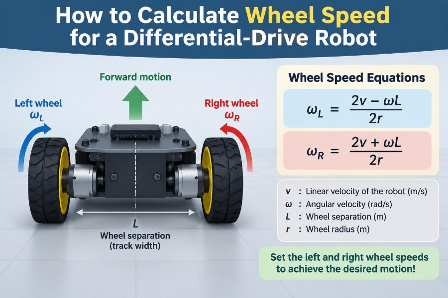
You need the effective wheel radius r and the track width L. Track width is the distance between the centers of the left and right wheel contact paths, not necessarily the outside width of the robot frame.
The effective radius is the radius that converts wheel rotation into actual travel. A nominal 70 mm wheel does not always have a 35 mm effective radius after tires, loading, compression, and manufacturing variation are considered.
🔄 Separate linear wheel speed from wheel rotation
“Wheel speed” can mean two different things. Linear wheel speed describes how fast the rim moves along the floor, usually in m/s. Rotational wheel speed describes how fast the wheel turns, in rad/s or revolutions per minute.
Keep these units distinct. The differential-drive geometry first gives left and right linear speeds; only afterward should you convert them to rotational motor commands.
📐 The core left and right wheel equations
For a reference point at the axle midpoint, the standard inverse-kinematics equations are:
v_left  = v - (ωL / 2)
v_right = v + (ωL / 2)
Here, v_left and v_right are linear speeds at the left and right wheel contact paths. The term ωL/2 is the extra speed one side needs, relative to the midpoint, to create the requested turn.
With positive ω defined as a left turn, the right wheel is faster. Reverse the signs if your coordinate convention defines positive rotation differently.
🎯 Understand why the equations work
During a turn, both wheels follow circular paths around one common instantaneous center of curvature. The outer wheel travels a larger circle than the inner wheel during the same time interval, so it must move farther and faster.
The midpoint path has radius R = v/ω when ω is not zero. The left and right path radii are R - L/2 and R + L/2, which leads directly to the core equations.
↩️ Calculate a straightforward turning example
Suppose a robot has a track width of L = 0.30 m. You command forward velocity v = 0.60 m/s and angular velocity ω = 1.00 rad/s.
v_left  = 0.60 - (1.00 × 0.30 / 2) = 0.45 m/s
v_right = 0.60 + (1.00 × 0.30 / 2) = 0.75 m/s
The robot turns left because its right wheel moves 0.30 m/s faster. Notice that the midpoint still advances at 0.60 m/s: the average of the two wheel speeds is (0.45 + 0.75)/2.
➡️ Recognize straight-line motion
Set ω = 0, and both equations reduce to v_left = v_right = v. This is the simplest test of an implementation: a straight command must produce identical values before any hardware-specific direction inversion is applied.
If equal commanded wheel speeds cause a curve, the calculation may be correct but the hardware is mismatched. Wheel radius, motor response, encoder scaling, friction, and chassis alignment can all contribute.
🌀 Command a turn in place
Set v = 0 while requesting a nonzero angular velocity. The wheels receive equal-magnitude, opposite-sign speeds:
v_left  = -ωL/2
v_right =  ωL/2
For a positive angular velocity, the left wheel reverses and the right wheel moves forward. This maneuver is useful in tight spaces, but it can cause tire scrub on high-grip surfaces because real wheels do not pivot without some lateral friction.
↪️ Know when one wheel stops
If v = ωL/2, the inner wheel speed becomes zero. The robot turns around that stationary wheel’s contact point, assuming the floor and wheel can support that idealized motion.
If |ωL/2| becomes larger than |v|, the inner wheel must reverse. That is not an error; it simply means the commanded curve is tighter than the geometry of a forward-only turn.
⭕ Connect speed commands to turning radius
For a smooth arc, radius at the midpoint is R = v/ω. This relationship is useful when a path planner specifies a radius rather than an angular rate.
You can substitute ω = v/R into the wheel equations. A larger radius produces wheel speeds closer together, while a smaller radius requires a larger difference between them.
⚙️ Convert linear speed to wheel angular velocity
Motor controllers and encoders often work in angular velocity. If a wheel has effective radius r, convert each linear wheel speed using:
Ω_left  = v_left / r
Ω_right = v_right / r
Ω is wheel angular velocity in rad/s. This equation assumes rolling without slip: each radian of wheel rotation advances the wheel by one radius length along the ground.
🔢 Convert radians per second to RPM
Many motor specifications use revolutions per minute. Convert angular velocity as follows:
RPM = Ω × 60 / (2π)For a wheel radius of 0.05 m moving at 0.50 m/s, Ω = 10 rad/s, which is about 95.5 RPM. Keep full precision in software and round only for display or interfaces that require integer commands.
🪛 Account for gear reduction correctly
A gearbox changes the relationship between motor shaft speed and wheel speed. If the reduction is 20:1, the motor rotates approximately 20 revolutions for each wheel revolution, ignoring losses and compliance.
Calculate wheel RPM first, then multiply by the gear ratio to estimate motor-shaft RPM. Do not multiply the wheel radius by the gear ratio; the wheel radius remains a physical property of the wheel.
📟 Translate speed into encoder counts
Closed-loop controllers often estimate speed from encoder counts. If an encoder provides N counts per wheel revolution after all decoding and gearing are considered, then a wheel rotating at RPM produces:
counts per second = RPM × N / 60Be precise about what N means. Quadrature encoders may be counted at different decoding resolutions, and an encoder mounted before a gearbox needs the gear ratio included in its wheel-revolution count.
🧮 Use one complete numerical example
Consider a hypothetical robot with wheel radius r = 0.05 m, track width L = 0.32 m, desired midpoint speed v = 0.40 m/s, and desired left-turn rate ω = 0.80 rad/s.
v_left  = 0.40 - (0.80 × 0.32 / 2) = 0.272 m/s
v_right = 0.40 + (0.80 × 0.32 / 2) = 0.528 m/s
Ω_left  = 0.272 / 0.05 = 5.44 rad/s
Ω_right = 0.528 / 0.05 = 10.56 rad/s
Converting the wheel rates gives approximately 52 RPM on the left and 101 RPM on the right. Those are wheel RPM values; a geared motor’s shaft RPM may be much higher.
📊 Keep units consistent from start to finish
Most silent wheel-speed failures are unit failures. Mixing millimeters with meters changes results by a factor of 1,000; mixing degrees per second with radians per second changes the turn term by roughly 57.3.
| Quantity | Recommended calculation unit | Common pitfall |
|---|---|---|
| Linear velocity | m/s | Using mm/s with dimensions in meters |
| Angular velocity | rad/s | Using degrees/s directly |
| Wheel radius and track width | m | Measuring frame width instead of wheel-center spacing |
| Rotational speed | rad/s or RPM | Confusing wheel and motor-shaft values |
🧱 Choose the correct reference point
The basic equations assume v is the velocity of the midpoint between the wheels. That is conventional, but a sensor, tool, or payload may be mounted ahead of that point.
A point offset forward by distance d moves sideways while the robot turns. If precision at an off-center tool matters, use rigid-body kinematics to transform the desired velocity at that tool back to the axle midpoint before calculating wheel speeds.
🧭 Apply a clear sign convention
Document which direction is positive for forward travel, left turns, and each motor’s shaft rotation. A robot with mirrored motors often needs one electrical command inverted even though the physical wheel-speed equations are unchanged.
Test signs safely with the wheels raised. A positive forward command should make both contact patches move toward the front of the robot; a positive turn command should produce the intended rotation direction.
🚧 Respect motor and wheel speed limits
Equations can request a wheel speed that the drivetrain cannot sustain. If the maximum allowable wheel linear speed is v_max, check whether either calculated wheel speed exceeds its magnitude.
Blindly clipping only the faster wheel changes both the robot’s average speed and curvature. A better approach is to scale both wheel commands by the same factor when preserving the requested path curvature matters.
📉 Scale commands without changing the curve
Let m = max(|v_left|, |v_right|). If m > v_max, multiply both wheel speeds by v_max/m.
The robot then travels more slowly, but the ratio between the wheel speeds remains the same. That preserves the intended curvature under the ideal kinematic model, although acceleration and traction may still limit the result.
⏱️ Limit acceleration as well as speed
A feasible final speed does not mean the robot can reach it instantly. Rapid changes in wheel speed demand torque, can break traction, stress gearboxes, and make a loaded robot overshoot.
Use acceleration limits or a velocity ramp for each wheel. In more demanding systems, jerk limiting—limiting how quickly acceleration changes—can improve mechanical smoothness and sensor stability.
🛞 Treat wheel radius as a calibration value
Measure effective radius by commanding a known number of wheel revolutions and measuring straight-line distance on the surface that matters. Divide distance by total wheel angle in radians to estimate the rolling radius.
Perform several trials in both directions. A radius estimated on carpet may differ from one measured on smooth vinyl because tire deformation and slip change the effective rolling behavior.
📐 Calibrate track width from turning behavior
Track width is also an effective kinematic parameter. A useful practical test is to command equal and opposite encoder-based wheel travel, measure the resulting robot rotation, and adjust the track-width value so predicted and measured angles agree.
This value may differ slightly from a caliper measurement. Tire scrub, wheel compliance, and the actual contact paths can make the effective turning width larger or smaller than the visible mechanical spacing.
🧊 Understand the no-slip assumption
The equations assume pure rolling: a wheel’s travel equals its rotation times radius, and neither wheel slides sideways. That approximation is often good enough at modest speeds on consistent flooring.
It becomes weaker during fast pivots, abrupt braking, travel on loose material, uneven loading, or a robot with high center of mass. Encoders still report wheel rotation during slip, so encoder-only odometry can confidently report motion the chassis did not make.
🧭 Combine encoders with other feedback
Encoders are excellent for regulating wheel speed and estimating short-term travel, but they do not directly measure the robot’s heading in the world. An IMU can help observe angular motion, while cameras, range sensors, or external localization can correct longer-term position drift.
Additional sensors do not replace correct wheel-speed kinematics. They complement it by detecting deviations caused by conditions the ideal model cannot capture.
🔁 Verify forward kinematics too
Inverse kinematics converts desired robot motion into wheel speeds. Forward kinematics checks the reverse relationship:
v = (v_right + v_left) / 2
ω = (v_right - v_left) / L
These equations are invaluable for unit tests. Feed a command into inverse kinematics, run the result through forward kinematics, and confirm that it reconstructs the original v and ω within numerical tolerance.
🧪 Test in a safe and useful sequence
Begin with wheels off the ground to check direction signs and encoder polarity. Then test low-speed straight travel, gentle constant-radius arcs, and slow turns in place on a clear floor.
- Mark a measured path and compare expected with observed distance.
- Command a known rotation and measure the actual heading change.
- Repeat tests at different battery levels and payloads.
- Log requested wheel speed, measured wheel speed, and pose estimates.
Logging reveals whether a problem originates in kinematics, motor control, saturation, or physical traction.
⚠️ Avoid common implementation mistakes
Several errors appear repeatedly in otherwise capable robot projects:
- Using wheel diameter where the formula requires radius.
- Using full track width in the turn term instead of
L/2. - Sending linear m/s values directly to a controller expecting RPM.
- Calculating in degrees/s without converting to rad/s.
- Clamping one wheel independently and unintentionally changing the path.
- Assuming nominal CAD dimensions are calibrated motion parameters.
Each mistake has a recognizable symptom, but symptoms can overlap. Work from units and definitions outward rather than tuning gains to hide a geometry error.
💻 Organize the calculation in software
Keep the geometry conversion separate from motor-control code. A small function should accept v, ω, L, and r, then return left and right wheel angular velocities in a documented unit.
Afterward, another layer can apply speed limits, acceleration limits, direction inversions, gear ratios, and encoder-controller conversions. Separation makes simulation, testing, and hardware changes far less error-prone.
🧰 Pseudocode for a robust command path
turn_term = omega * track_width / 2
left_linear  = v - turn_term
right_linear = v + turn_term

scale = max(1, abs(left_linear)/max_wheel_speed,
                abs(right_linear)/max_wheel_speed)
left_linear  = left_linear / scale
right_linear = right_linear / scale

left_wheel_rad_s  = left_linear / wheel_radius
right_wheel_rad_s = right_linear / wheel_radius

apply_acceleration_limits()
send_closed_loop_speed_commands()
The order is deliberate: calculate geometry first, preserve curvature when scaling, convert to rotational units, then shape the command for real hardware.
🧠 Match the model to the mission
For a small indoor teaching robot moving slowly, the basic equations plus encoder feedback may be entirely adequate. For a fast vehicle, heavy payload, rough terrain, or high-accuracy docking task, the same equations remain the starting point but require better calibration, sensing, and dynamic control.
Do not mistake a kinematic model for a complete physical model. Kinematics describes the motion implied by geometry; dynamics determines whether motors, friction, mass, and power can actually produce it.
✅ Bring the calculation back to one core principle
A differential-drive robot turns because its wheels cover different distances in the same time. The wheel-speed difference sets angular motion, while their average sets forward motion.
Start from desired midpoint velocity and angular velocity, use the measured track width to find left and right linear speeds, then use effective wheel radius to convert those values into rotational motor targets. Calibrate the dimensions, enforce practical limits, and verify behavior on the real surface.
Reliable differential-drive motion comes from pairing simple geometry with honest measurements and feedback from the actual robot. With that foundation, a straight line, a smooth arc, and a precise rotation all become understandable commands rather than trial-and-error motor settings. 🦾🧭⚙️