
Target point manipulation inside a deformable object by a robotic system is necessary in many medical and industrial applications such as breast biopsy, drug injection, suturing, precise machining of deformable objects etc. However, this is a challenging problem because of the difficulty of imposing the motion of the internal target point by a finite number of actuation points located at the boundary of the deformable object. In addition, there exist several other important manipulative operations that deal with deformable objects such as whole body manipulation [1], shape changing [2], biomanipulation [3] and tumor manipulation [4] that have practical applications. The main focus of this chapter is the target point manipulation inside a deformable object. For instance, a positioning operation called linking in the manufacturing of seamless garments [5] requires manipulation of internal points of deformable objects. Mating of a flexible part in electric industry also results in the positioning of mated points on the object. In many cases these points cannot be manipulated directly since the points of interest in a mating part is inaccessible because of contact with a mated part.
Additionally, in medical field, many diagnostic and therapeutic procedures require accurate needle targeting. In case of needle breast biopsy [4] and prostate cancer brachytherapy [6], needles are used to access a designated area to remove a small amount of tissue or to implant radio-active seed at the targeted area. The deformation causes the target to move away from its original location. To clarify the situation we present a schematic of needle insertion for breast biopsy procedure as shown in Figure 1. When tip of the needle reaches the interface between two different types of tissue, its further insertion will push the tissue, instead of piercing it, causing unwanted deformations. These deformations move the target away from its original location as shown in Figure 1(b). In this case, we cannot manipulate the targeted area directly because it is internal to the organ. It must be manipulated by controlling some other points where forces can be applied as shown in Figure 1(c). Therefore, in some cases one would need to move the positioned points to the desired locations of these deformable objects (e.g., mating two deformable parts for sewing seamlessly) while in other cases one may need to preserve the original target location (e.g., guiding the tumor to fall into the path of needle insertion). In either of these situations, the ability of a robotic system to control the target of the deformable object becomes important, which is the focus of this chapter.
To control the position of the internal target point inside a deformable object requires appropriate contact locations on the surface of the object. Therefore, we address the issue of determining the optimal contact locations for manipulating a deformable object such that the internal target point can be positioned to the desired location by three robotic fingers using minimum applied forces. A position-based PI controller is developed to control the motion of the robotic fingers such that the robotic fingers apply minimum force on the surface of the object to position the internal target point to the desired location. However, the controller for target position control is non-collocated since the internal target point is not directly actuated by the robotic fingers. It is known in the literature that non-collocated control of a deformable object is not passive, which may lead to instability [7]. In order to protect the object and the robotic fingers from physical damage and also in order to diminish the deterioration of performance caused by unwanted oscillation, it is indispensable to build stable interaction between the robotic fingers and the object. Here we consider that the plant (i.e., the deformable object) is passive and does not generate any energy. So, in order to have stable interaction, it is essential that the controller for the robotic fingers must be stable. Thus, we present a new passivity-based non-collocated controller for the robotic fingers to ensure safe and accurate position control of the internal target point. The passivity theory states that a system is passive if the energy flowing in exceeds the energy flowing out. Creating a passive interface adds the required damping force to make the output energy lower than the input energy. To this end we develop a passivity observer (PO) and a passivity controller (PC) based on [8] for individual robotic finger where PO monitors the net energy flow out of the system and PC will supply the necessary damping force to make PO positive. Our approach extends the concept of PO and PC in [8] to multi- point contacts with the deformable object.

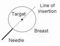
(a) (b) (c)
Fig. 1. Schematics of needle breast biopsy procedure: (a) needle insertion, (b) target movement, and (c) target manipulation
The remainder of this chapter is organized as follows: we discuss various issues and prior research in Section 2. The problem description is stated in Section 3. Section 4 outlines the mathematical modelling of the deformable object. A framework for optimal contact locations is presented in Section 5. The control methods are discussed in Section 6. The effectiveness of the derived control law is demonstrated by simulation in Section 7. Finally, the contributions of this work and the future directions are discussed in Section 8.
Issues and prior research
A considerable amount of work on multiple robotic systems has been performed during the last few decades [9-11, 12-15]. Mostly, the position and/or force control of multiple manipulators handling a rigid object were studied in [9-11]. However, there were some works on handling deformable object by multiple manipulators presented in [12-15]. Saha and Isto [12] presented a motion planner for manipulating deformable linear objects using two cooperating robotic arms to tie self-knots and knots around simple static objects. Zhang et al. [13] presented a microrobotic system that is capable of picking up and releasing operation of microobjects. Sun et al. [14] presented a cooperation task of controlling the reference motion and the deformation when handling a deformable object by two manipulators. In [15], Tavasoli et al. presented two-time scale control design for trajectory tracking of two cooperating planar rigid robots moving a flexible beam. However, to the best of our knowledge the works on manipulating an internal target point inside a deformable object are rare [4, 5]. Mallapragada et al. [4] developed an external robotic system to position the tumor in image-guided breast biopsy procedures. In their work, three linear actuators manipulate the tissue phantom externally to position an embedded target inline with the needle during insertion. In [5] Hirai et al. developed a robust control law for manipulation of 2D deformable parts using tactile and vision feedback to control the motion of the deformable object with respect to the position of selected reference points. These works are very important to ours present application, but they did not address the optimal locations of the contact points for effecting the desired motion.
A wide variety of modeling approaches have been presented in the literature dealing with computer simulation of deformable objects [16]. These are mainly derived from physically- based models to produce physically valid behaviors. Mass-spring models are one of the most common forms of deformable objects. A general mass-spring model consists of a set of point masses connected to its neighbors by massless springs. Mass-spring models have been used extensively in facial animation [17], cloth motion [18] and surgical simulation [19]. Howard and Bekey [20] developed a generalized method to model an elastic object with the connections of springs and dampers. Finite element models have been used in the computer simulation to model facial tissue and predict surgical outcomes [21, 22]. However, the works on controlling an internal point in a deformable object are not attempted.
In order to manipulate the target point to the desired location, we must know the appropriate contact locations for effecting the desired motion. There can be an infinite number of possible ways of choosing the contact location based on the object shapes and task to be performed. Appropriate selection of the contact points is an important issue for performing certain tasks. The determination of optimal contact points for rigid object was extensively studied by many researchers with various stability criteria. Salisbury [23] and Kerr [24] discussed that a stable grasp was achieved if and only if the grasp matrix is full row rank. Abel et al. [25] modelled the contact interaction by point contact with Coulomb friction and they stated that optimal grasp has minimum dependency on frictional forces. Cutkosky [26] discussed that the size and shape of the object has less effect on the choice of grasp than by the tasks to be performed after examining a variety of human grasps. Ferrari et al. [27] defined grasp quality to minimize either the maximum value or sum of the finger forces as optimality criteria. Garg and Dutta [28] shown that the internal forces required for grasping deformable objects vary with size of object and finger contact angle. In [29], Watanabe and Yoshikawa investigated optimal contact points on an arbitrary shaped object in 3D using the concept of required external force set. Ding et al. proposed an algorithm for computing form closure grasp on a 3D polyhedral object using local search strategy in [30]. In [31, 32], various concepts and methodologies of robot grasping of rigid objects were reviewed. Cornella et al. [33] presented a mathematical approach to obtain optimal solution of contact points using the dual theorem of nonlinear programming. Saut et al. [34] presented a method for solving the grasping force optimization problem of multi-fingered dexterous hand by minimizing a cost function. All these works are based on grasp of rigid objects.
There are also a few works based on deformable object grasping. Like Gopalakrishnan and Goldberg [35] proposed a framework for grasping deformable parts in assembly lines based on form closure properties for grasping rigid parts. Foresti and Pellegrino [36] described an automatic way of handling deformable objects using vision technique. The vision system worked along with a hierarchical self-organizing neural network to select proper grasping points in 2D. Wakamatsu et al. [37] analyzed grasping of deformable objects and introduced bounded force closure. However, position control of an internal target point in a deformable object by multi-fingered gripper has not been attempted. In our work, we address the issue of determining the optimal contact locations for manipulating a deformable object such that the internal target point can be positioned to the desired location by three robotic fingers using minimum applied forces.
The idea of passivity can be used to guarantee the stable interaction without exact knowledge of model information. Anderson and Spong [38] published the first solid result by passivation of the system using scattering theory. A passivity based impedance control strategy for robotic grasping and manipulation was presented by Stramigioli et al. [39]. Recently, Hannaford and Ryu [40] proposed a time-domain passivity control based on the energy consumption principle. The proposed algorithm did not require any knowledge about the dynamics of the system. They presented a PO and a PC to ensure stability under a wide variety of operating conditions. The PO can measure energy flow in and out of one or more subsystems in real-time by confining their analysis to system with very fast sampling rate. Meanwhile the PC, which is an adaptive dissipation element, absorbs exactly net energy output measured by the PO at each time sample. In [41], a model independent passivity-based approach to guarantee stability of a flexible manipulator with a non- collocated sensor-actuator pair is presented. This technique uses an active damping element to dissipate energy when the system becomes active. In our work we use the similar concept of PO and PC to ensure stable interaction between the robotic fingers and the deformable object. Our work also extends the concept of PO and PC for multi-point contact with the deformable object.
Problem description
Consider a case in which multiple robotic fingers are manipulating a deformable object in a 2D plane to move an internal target point to a desired location. Before we discuss the design of the control law, we present a result from [42] to determine the number of actuation points required to position the target at an arbitrary location in a 2D plane. The following definitions are given according to the convention in [42].
Manipulation points: are defined as the points that can be manipulated directly by robotic fingers. In our case, the manipulation points are the points where the external robotic fingers apply forces on the deformable object.
Positioned points: are defined as the points that should be positioned indirectly by controlling manipulation points appropriately. In our case, the target is the position point. The control law to be designed is non-collocated since the internal target point is not directly actuated by the robotic fingers. The following result is useful in determining the number of actuation points required to accurately position the target at the desired location.
Result [42]: The number of manipulated points must be greater than or equal to that of the positioned points in order to realize any arbitrary displacement.
In our present case, we assume that the number of positioned points is one, since we are trying to control the position of the target. Hence, ideally the number of contact points would also be one. But practically, we assume that there are two constraints: (1) we do not want to apply shear force on the deformable object to avoid the damage to the surface, and (2) we can only apply control force directed into the deformable object. We cannot pull the surface since the robotic fingers are not attached to the surface. Thus we need to control the position of the target by applying only unidirectional compressive force.
In this context, there exists a theorem on the force direction closure in mechanics that helps
us determining the equivalent number of compressive forces that can replace one unconstrained force in a 2D plane.
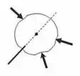
Theorem [43]: A set of wrenches w can generate force in any direction if and only if there
exists a three-tuple of wrenches {w1 , w2 , w3 }
satisfy:
whose respective force directions
f1 ,
f2 , f3
i. Two of the three directions f1 , f2 , f3 are independent
ii. A strictly positive combination of the three directions is zero.
α f1 + β f2 + γ f3 = 0
(1)
where α , β , and γ are constants. The ramification of this theorem for our problem is that we need three control forces distributed around the object such that the end points of their direction vectors draw a non-zero triangle that includes their common origin point. With such an arrangement we can realize any arbitrary displacement of the target point. Thus the problem can be stated as:
Problem statement: Given the number of actuation points, the initial target and its desired
locations, find appropriate contact locations and control action such that the target point is positioned to its desired location by controlling the boundary points of the object with minimum force.
Deformable object modelling
Consider a schematic in Figure 2 where three robotic fingers are positioning an internal target (point A) in a deformable object to the desired location (point B). We assume that all the end-effectors of the robotic fingers are in contact with the deformable object such that they can apply only push on the object as needed.
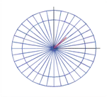
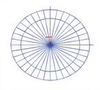
The coordinate systems are defined as follows: w is the task coordinate system, o is the object coordinate system, fixed on the object and i is the i-th robotic finger coordinate system, fixed on the i-th end-effectors located at the grasping point. In order to formulate the optimal contact locations, we model the deformable object using mass-spring-damper systems. The point masses are located at the nodal points and a Voigt element [20] is inserted between them. Figure 3 shows a single layer of the deformable object. Each element is labeled as Ej for j = 1, 2 , , NE where NE is total number of elements in a single layer.
| i i i |
Position vector of the i-th mesh point is defined as p = [x y ]T , i = 1, 2, 3,…, N where, N
is total number of point masses. k and c are the spring stiffness and the damping coefficient, respectively. Assume that no moment exerts on each mesh point. Then, the resultant force exerted on the mesh point, pi , can be calculated

where, U denotes the total potential energy of the object
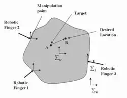
Fig. 2. Schematic of the robotic fingers manipulating a deformable object
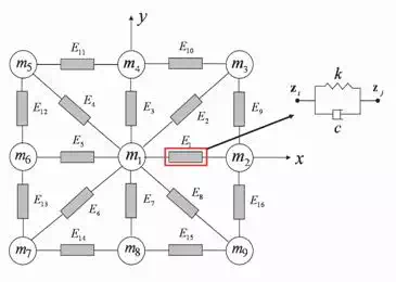
Fig. 3. Model of a deformable object with interconnected mass-spring-damper
Framework for optimal contact locations
We develop an optimization technique that satisfies the force closure condition for three fingers planar grasp. The resultant wrench for the contacts of three robotic fingers is given by
where, ni ( ri )
is the unit inner normal of i-th contact and
fi denotes the i-th finger’s force.
We assume that the contact forces should exist in the friction cone to manipulate objects without slip of the fingertip. Now we need to find three distinct points, r1 (θ1 ) , r2 (θ2 ) , and r3 (θ3 ) , on the boundary of the object such that Equation (3) is satisfied. Here, θ1 , θ2 , and θ3 are the three contact point locations measured anti-clockwise with respect to the x axis as
shown in Figure 4. In addition, we assume that the normal forces have to be non-negative to avoid separation and slippage at the contact points, i.e.,
fi ≥ 0 , i = 1, 2, 3
(4)
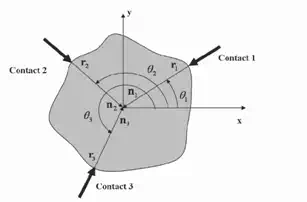
Fig. 4. Three fingers grasp of a planar object
A physically realizable grasping configuration can be achieved if the surface normals at three contact points positively span the plane so that they do not all lie in the same half- plane [44]. Therefore, a realizable grasp can be achieved if the pair-wise angles satisfy the following constraints
θmin ≤|θi − θ j |≤ θmax , θlow ≤ θi ≤ θhigh , i , j = 1, 2 , 3 , i ≠ j (5)
A unique solution to realizable grasping may not always exist. Therefore, we develop an optimization technique that minimizes the total force applied on to the object to obtain a particular solution. The optimal locations of the contact points would be the solution of the following optimization problem.
min fT f
sunject to
3
w = fi ni (ri )
i = 1
![]()
![]() θmin ≤ θi − θ j ≤ θmax , i , j = 1, 2 , 3 , i ≠ j fi ≥ 0 , i = 1, 2, 3
θmin ≤ θi − θ j ≤ θmax , i , j = 1, 2 , 3 , i ≠ j fi ≥ 0 , i = 1, 2, 3
| i |
0 ≤ θ ≤ 360 , i = 1, 2, 3
(6)
Once we get the optimal contact locations, all three robotic fingers can be located at their respective positions to effect the desired motion at those contact points.
Design of the controller
In this section, a control law for the robotic fingers is developed to guide a target from any point A to an arbitrary point B within the deformable object as shown in Figure 2.
Target position control
At any given time-step, point A is the actual location of the target and point B is the desired location of the target. n1, n2 and n3 are unit vectors which determine the direction of force application of the actuation points with respect to the global reference frame w . Let assume, pd is the position vector of point B and p is the position vector of point A. Referring to Figure 2, the position vector of point A is given by

where, x and y are the position coordinates of point A in the global reference frame w . The desired target position is represented by point B whose position vector is given b
| d d d |
p = [x y ]T
(8)
where, xd and yd
given by
are the desired target position coordinates. The target position error, e, is
e = pd − p
(9)
Once the optimal contact locations are determined from Equation (6), the planner generates the desired reference locations for these contact points by projecting the error vector between the desired and the actual target locations in the direction of the applied forces, which is given by

where,

All robotic fingers are controlled by their individual controllers using the following proportional-integral (PI) control law

where,
KPi , and
KIi
are the proportional and integral gains. Note that in the control law (12), mechanical properties of the deformable object are not required. Forces applied by the fingers on the surface of the deformable object are calculated by projecting the error vector in the direction of the applied forces. But the Equation (12) does not guarantee that the system will be stable. Thus a passivity-based control approach based on energy monitoring is developed to guarantee the stability of the system.
Passivity-based control
A passivity-based control approach based on energy monitoring is developed for deformable object manipulation to guarantee passivity (and consequently stability) of the system. The main reason to use passivity-based control is to ensure stability without the need of having an accurate model of the deformable object. It is not possible to develop a precise dynamic model of a deformable object due to complex nonlinear internal dynamics as well as variation in geometry and mechanical properties. Thus passivity based control is an ideal candidate to ensure stability since it is a model independent technique. The basic idea is to use a PO to monitor the energy generated by the controller and to dissipate the excess energy using a PC when the controller becomes active [41], without the need for modeling the dynamics of the plant (deformable object).
Passivity Observer (PO)
We develop a network model with PO and PC similar to [41] as shown in Figure 5. The PO monitors the net energy flow of the individual finger’s controller. When the energy becomes negative, PC dissipates excess energy from the individual controller. Similar to [41] energy is defined as the integral of the inner product between conjugate input and output, which may or may not correspond to physical energy. Definition of passivity [41] states that the energy applied to a passive network must be positive for all time. Figure 5 shows a network representation of the energetic behavior of this control system. The block diagram in Figure
5 is partitioned into three elements: the trajectory generator, the controller and the plant. Each controller corresponds to one finger. Since three robotic fingers are used for planar manipulation, three individual controller transfer energy to the plant.
The connection between the controller and the plant is a physical interface at which
conjugate variables ( fi , vi ; where fi is the force applied by i-th finger and vi is the velocity of i-th finger) define physical energy flow between controller and plant. The forces and velocities are given by
| 1 2 3 |
f = [ f f f ]T
(13)
| 1 2 3 |
v = [v v v ]T
(14)
The desired target velocity is obtained by differentiating (8) with respect to time and is given by

where, x d
and y d
are the desired target velocities, respectively. The desired target velocity along the direction of actuation of the i-th robotic finger is given by
vdi = p d ⋅ ni
(16)
The trajectory generator essentially computes the desired target velocity along the direction of actuation of the robotic fingers. If the direction of actuation of the robotic fingers, ni , and
desired target velocity,
p d , are known with respect to a global reference frame then the
trajectory generator computes the desired target velocity along the direction of actuation of the fingers using Equation (16).
The connections between the trajectory generator and the controller, which traditionally consist of a one-way command information flow, are modified by the addition of a virtual feedback of the conjugate variable [41]. For the system shown in Figure 5, output of the
trajectory generator is the desired target velocity,
vdi , along direction of i-th finger and
output of the controller is calculated from Equation (12).
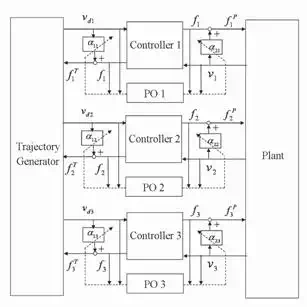
Fig. 5. Network representation of the control system. α1i and α2 i are the adjustable damping elements at each port, i=1,2,3
For both connections, virtual feedback is the force applied by the robotic fingers. Integral of the inner product between trajectory generator output ( vdi ) and its conjugate variable ( fi ) defines “virtual input energy.” The virtual input energy is generated to give a command to the controller, which transmits the input energy to the plant through the controller in the form of “real output energy.” Real output energy is the physical energy that enters to the plant (deformable object) at the point where the robotic finger is in contact with the object. Therefore, the plant is a three-port system since three fingers manipulate the object. The
conjugate pair that represents the power flow is fi , vi (the force and the velocity of i-th finger, respectively). The reason for defining virtual input energy is to transfer the source of energy from the controllers to the trajectory generator. Thus the controllers can be represented as two-ports which characterize energy exchange between the trajectory generator and the plant. Note that the conjugate variables that define power flow are discrete time values and so the analysis is confined to systems having a sampling rate substantially faster than the system dynamics.
For regulating the target position during manipulation,
vdi = 0 . Hence the trajectory generator is passive since it does not generate energy. However, for target tracking, vdi ≠ 0 and fi ≠ 0 . Therefore the trajectory generator is not passive because it has a velocity source as a power source. It is shown that even if the system has an active term, stability is guaranteed as long as the active term is not dependent on the system states [45]. Therefore, passivity of the plant and controllers is sufficient to ensure system stability.
Here, we consider that the plant is passive. Now we design a PO for sufficiently small time- step ΔT as:
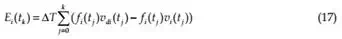
where, ΔT is the sampling period and
t j = j × ΔT . In normal passive operation,
Ei (t j )
should always be positive. In case when Ei (t j ) < 0 , the PO indicates that the i-th controller is generating energy and going to be active. The sufficient condition to make the whole system passive can be written as
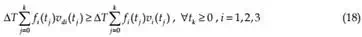
where k means the k-th step sampling time.
The active and passive port can be recognized by monitoring the conjugate signal pair of each port in real time. A port is active if
fv < 0 that means energy is flowing out of the network system and it is passive if fv ≥ 0 , that means energy is flowing into the network system. The input and output energy can be computed as [46]
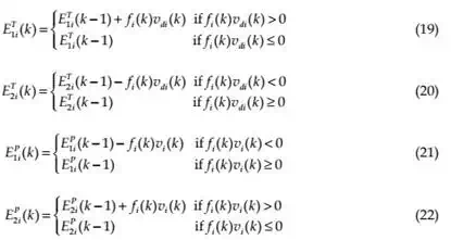
where,
| 1i |
ET (k) and
| 2 i |
ET (k) are the energy flowing in and out at the trajectory side of theP Pcontroller port, respectively, whereas E1i (k) and E2 i (k) are the energy flowing in and out at the plant side of the controller port, respectively. So the time domain passivity condition is given by

Net energy output of an individual controller is given by
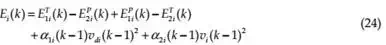
where, the last two terms are the energy dissipated at the previous time step. α1i (k − 1) and
α2 i (k − 1) are the damping coefficient calculated based on PO discussed below.
Passivity Controller (PC)
In order to dissipate excess energy of the controlled system, a damping force should be applied to its moving parts depending on the causality of the port. As it is well known, such a force is a function of the system’s velocities giving the physical damping action on the system. Mathematically, the damping force is given by
f d = α v
(25)
where α is the adjustable damping factor and v is the velocity. From this simple observation, it seems necessary to measure and use the velocities of the robotic fingers in the control algorithm in order to enhance the performance by means of controlling the damping forces acting on the systems. On the other hand, velocities measurements are not always available and in these cases position measurements can be used to estimate velocities and therefore to inject damping.
When the observed energy becomes negative, the damping coefficient is computed using the following relation (which obeys the constitutive Equation (25)). Therefore, the algorithm used for a 2-port network with impedance causality (i.e., velocity input, force output) at each port is given by the following steps:

P
| i |
| i |
where, f t (k) and f p (k ) are the PCs’ outputs at trajectory and plant sides of the controller
| i |
| i |
ports, respectively. f T (k) and f P (k ) are the modified outputs at trajectory and plant sides![]()
![]()
![]()
![]() of the controller ports, respectively.
of the controller ports, respectively.
Simulation and discussion
We perform extensive simulations of positioning an internal target point to a desired location in a deformable object by external robotic fingers to demonstrate the feasibility of the concept. We discretize the deformable object with elements of mass-spring-damper. We choose m=0.006 kg for each point mass, k=10 N/m for spring constant and c=5 Ns/m for damping coefficient. With this parameter set up, we present four different simulation tasks.
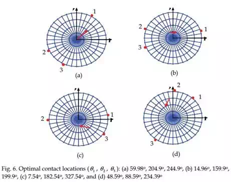
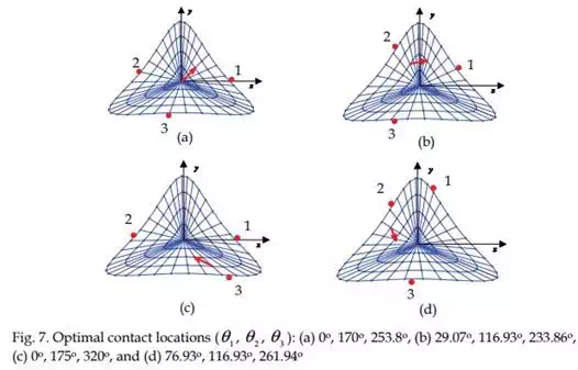
Task 1:
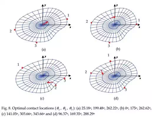
In Task 1, we present the optimal contact locations of various objects using three robotic fingers such that an internal target point is positioned to the desired location with minimum force. The optimal contact locations are computed using Equation (6) as shown in Figures 6 to 8. In these figures, the base of the arrow represents the initial target location and the arrow head denotes the desired location of the target point. The contact locations are depicted by the bold red dots on the periphery of the deformable object. Note that in determining the optimal contact locations, we introduced minimum angle constraints between any two robotic fingers to achieve a physically realizable grasping configuration.
 |
Task 2:
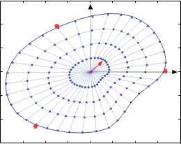
In Task 2, we present a target positioning operation when the robotic fingers are not located at their optimal contact locations. For instance, we choose that the robotic fingers are located at 0, 120, and 240 degrees with respect to the x-axis as shown in Figure 9. We assume that the initial position of the target is at the center of the section of the deformable object, i.e., (0, 0) mm. The goal is to position the target at the desired location (5, 5) mm with a smooth
0.06
 y
y
0.04 2
0.02
1
![]() 0
0
x
-0.02
-0.04
3
–0.06
-0.04 -0.03 -0.02 -0.01 0 0.01 0.02 0.03 0.04
x (m)
Fig. 9. Deformable object with contact points located at 0, 120 and 240 degrees with respect to x-axis
6
5
4
![]() 3
3
2
1
![]()
![]() desired actual
desired actual
0
0 1 2 3 4 5 6
x (mm)
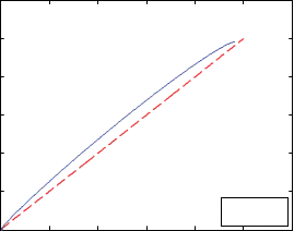
Fig. 10. The desired (red dashed) and the actual (blue solid) straight lines when robotic fingers are located at 0, 120, and 240 degrees with respect to x-axis straight line trajectory. In this simulation, we choose KPi =1000 and KIi =1000, i=1,2,3. Figure
| f1 f2f3 |
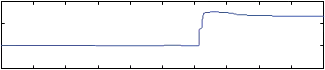
10 shows the actual and desired position trajectories of the target point. It is noticed that there is some error present in the tracking of the desired trajectory. Robotic fingers forces generated by the PI controller are presented in Figure 11 and the POs are falling to negative as shown in Figure 12. Negative values of POs signify that the interaction between the robotic fingers and the deformable object is not stable.
1.8
1.6
![]() 1.4
1.4
![]() 1.2
1.2
1
0.8
0.6
0.4
0.2
 0
0
0 1 2 3 4 5 6 7 8 9 10 time (sec.)
Fig. 11. Controller forces when robotic fingers are located at 0, 120, and 240 degrees with respect to x-axis
0.01
![]() 0
0
-0.01
0.01
 0 1 2 3 4 5 6 7 8 9 10
0
![]() -0.01
-0.01
-0.02
0.05
 0 1 2 3 4 5 6 7 8 9 10
![]() 0
0
-0.05
 0 1 2 3 4 5 6 7 8 9 10 time (sec.)
Fig. 12. POs when robotic fingers are located at 0, 120, and 240 degrees with respect to x-axis
Task 3:
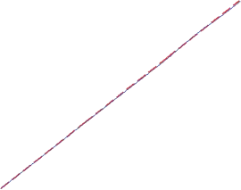
In Task 3, we consider the same task as discussed above under Task 2 but the robotic fingers are positioned at their optimal contact locations (Figure 8(a)) and the target is following the desired straight line trajectory. In this case, PCs are not turned on while performing the task. A simple position based PI controller generates the control command based on the error between the desired and the actual location of the target. Figure 13 shows that the target
6
5
4
![]() 3
3
2
1
 desired actual
0
0 1 2 3 4 5 6
x (mm)
Fig. 13. The desired (red dashed) and the actual (blue solid) straight lines when PCs are not turned on
0.8
![]() f
f
1
0.7 f
 2
2
f
0.6 3
![]() 0.5
0.5
0.4
0.3
0.2
0.1
0
-0.1
0 1 2 3 4 5 6 7 8 9 10 time (sec.)
Fig. 14. Controller forces when PCs are not turned on
0.01
![]() 0
0
-0.01
5
 0 1 2 3 4 5 6 7 8 9 10
-3
 x 10
x 10
![]() 0
0
-5
0 1 2 3 4 5 6 7 8 9 10
-3
 x 10
x 10
5
![]() 0
0
-5
 0 1 2 3 4 5 6 7 8 9 10
time (sec.)
(a)
0.01
![]()
![]() 0
0
-0.01
1
0 0.1 0.2 0.3 0.4 0.5 0.6 0.7 0.8 0.9 1
-6
 x 10
x 10
![]() 0
0
-1
0 0.1 0.2 0.3 0.4 0.5 0.6 0.7 0.8 0.9 1
-7
 x 10
x 10
5
![]() 0
0
-5
0 0.1 0.2 0.3 0.4 0.5 0.6 0.7 0.8 0.9 1
time (sec.)
(b)
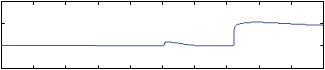
Fig. 15. (a) POs for three robotic fingers when PCs are not turned on, (b) a magnified version of (a) for first few seconds
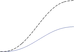
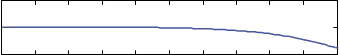
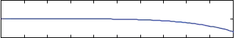
tracked the desired position trajectory. Robotic fingers forces generated by the PI controller are presented in Figure 14. Force values in Figure 14 are quite less than those in Figure 11 because of the optimal contact location of the robotic fingers. However, the POs for robotic fingers 2 and 3 are become negative as shown in Figure 15. Negative values of the POs signify that the output energy of the 2-port network is greater than the input energy. Since the plant is considered to be passive, the only source of generating extra energy is the controller that makes the whole system unstable. So we must engage passivity controller to modify the controller output by dissipating the extra amount of energy.
Task 4:
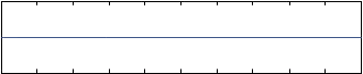
![]() In Task 4, the PCs are turned on and the robotic fingers are commanded to effect the desired motion of the target. The PCs are activated when the POs cross zero from a positive value. The required damping forces are generated to dissipate only the excess amount of energy generated by the controller. In this case, the target tracks the desired straight line trajectory well with the POs remaining positive. Figure 16 represents the actual and the desired trajectories of the target when PCs are turned on. For this case, the PCs on the plant side are only activated whereas the PCs on the trajectory side remain idle. Figure 17 shows the PCs forces generated at the plant side when the POs cross zero. The POs become positive during interaction between the robotic fingers and the object as shown in Figure 18. Hence, the stability of the overall system is guaranteed. The PCs on the trajectory side are shown in Figure 19, which are all zeros. The modified controller outputs to move the target point are shown in Figure 20.
In Task 4, the PCs are turned on and the robotic fingers are commanded to effect the desired motion of the target. The PCs are activated when the POs cross zero from a positive value. The required damping forces are generated to dissipate only the excess amount of energy generated by the controller. In this case, the target tracks the desired straight line trajectory well with the POs remaining positive. Figure 16 represents the actual and the desired trajectories of the target when PCs are turned on. For this case, the PCs on the plant side are only activated whereas the PCs on the trajectory side remain idle. Figure 17 shows the PCs forces generated at the plant side when the POs cross zero. The POs become positive during interaction between the robotic fingers and the object as shown in Figure 18. Hence, the stability of the overall system is guaranteed. The PCs on the trajectory side are shown in Figure 19, which are all zeros. The modified controller outputs to move the target point are shown in Figure 20.
6
5
4
![]() 3
3
2
1
| desired actual |
0
 0 1 2 3 4 5 6
![]() x (mm)
x (mm)
Fig. 16. The desired (red dashed) and the actual (blue solid) straight lines when PCs are turned on
0.1
![]()
![]() 0
0
-0.1
0.4
 0 1 2 3 4 5 6 7 8 9 10
![]()
![]() 0.2
0.2
0
0.4
 0 1 2 3 4 5 6 7 8 9 10
![]()
![]() 0.2
0.2
0
 0 1 2 3 4 5 6 7 8 9 10
time (sec.)
Fig. 17. Required forces supplied by PCs at the plant side when PCs are turned on
0.01
![]() 0
0
-0.01
0.2
 0 1 2 3 4 5 6 7 8 9 10
![]() 0.1
0.1
![]() 0
0
-0.1
0.02
 0 1 2 3 4 5 6 7 8 9 10
![]() 0.01
0.01
0
-0.01
 0 1 2 3 4 5 6 7 8 9 10 time (sec.)
Fig. 18. POs for three robotic fingers when PCs are turned on
1
![]()
![]() 0
0
-1
 0 1 2 3 4 5 6 7 8 9 10
1
![]()
![]() 0
0
-1
 0 1 2 3 4 5 6 7 8 9 10
1
![]()
![]() 0
0
-1
0 1 2 3 4 5 6 7 8 9 10
time (sec.)
Fig. 19. PCs forces at the trajectory side when PCs are turned on
0.8
![]() fP
fP
0.7 1
![]() fP
fP
2
0.6 fP
 3
3
![]() 0.5
0.5
0.4
0.3
0.2
0.1
0
-0.1
0 1 2 3 4 5 6 7 8 9 10 time (sec.)
Fig. 20. Modified controller forces when PCs are turned on
Conclusion and future work
In this chapter, an optimal contact formulation and a control action are presented in which a deformable object is manipulated externally by three robotic fingers such that an internal target point is positioned to the desired location. First, we formulated an optimization technique to determine the contact locations around the periphery of the object so that the target can be manipulated with minimum force applied on the object. The optimization technique considers a model of the deformable object. However, it is difficult to build an exact model of the deformable object in general due to nonlinear elasticity, friction, parameter variations, and other uncertainties. Therefore, we considered a coarse model of the deformable object to determine the optimal contact locations which is more realizable. A time-domain passivity control scheme with adjustable dissipative elements has been developed to guarantee the stability of the whole system. Extensive simulation results validate the optimal contact formulation and stable interaction between the robotic fingers and the object.