Robots are currently being designed based on human morphologies. Therefore, the most recent humanoid robots are technologically complex systems, with an extremely high level of mechanical and electronic integration. They are equipped with complete perceptive systems, which enable them to interact with the human beings and to move in human environments. However, controlling humanoid robots is difficult, particularly walking motions and balance when walking, during transitions from walking to stopping, or when the robot undergoes external thrusts. The walking and running abilities of humans have caused researchers to focus on muscular skeletal system properties, with a focus on improving the walking and interaction capabilities of robots.
One of the most significant properties of the mammalian muscle is compliance, that is, the capacity to adapt the muscle stiffness to various movements and interactions. When walking, the muscular compliance is implicated at a low level of control because it occurs in the muscle (the actuator) according to the required movement of the limb. Muscle compliance allows a muscle to optimize energy consumption by storing energy in passive phases and restoring energy for active phases. This intrinsic muscle stiffness control allows humans to run, walk, control walk‐halt‐walk transitions, and control posture related to external perturbations (other systems, such as the vestibular apparatus, are also involved in balancing, walking, and running processes).
RECENT PROGRESS IN ARTICULAR COMPLIANCE FOR LEGGED ROBOTS
Creating an artificial system that can mimic mammalian muscle behavior would represent significant progress in the field of humanoid robots. This goal can be achieved via numerous advancements.
COMPLIANT ACTUATORS
Special mechanical systems can be built that store and restore energy based on the walking phases. This approach, which is known as passive dynamic walking, was pioneered by McGeer more than a decade ago and has been analyzed by several studies. Passive dynamic walking is attractive due to its elegance and simplicity. However, active feedback control is necessary to achieve walking on the ground and varying slopes, for robustness related to uncertainties and disturbances, and to regulate the walking speed. The first active feedback control that exploits passive walking appeared for planar bipeds. Three‐dimensional (3‐D) passive walking was studied, the results of which were extended to the general case of 3‐D walking. An interesting extension of these concepts uses geometric reduction methods to generate stable 3‐D walking from two‐dimensional (2‐D) gaits. Robustness issues were addressed by using total energy as a storage function in the hybrid passivity framework.
Another manner in which to achieve compliance is to design actuators that reproduce the properties of mammalian muscles. These novel elastic actuators can be regarded as an artificial “muscle‐tendon”. The McKibben pneumatic muscle actuator produces a high force at low speeds, but these actuators are difficult to control because of their nonlinearity depending on air temperature and pressure. However, artificial pneumatic muscles or elastic actuators can be used to actuate joints of bipedal robot and their natural compliance improves robustness to postural and motion in jumping experiments.
Alternatives, such as piezoelectric actuator, electroactive polymers, or shape memory alloys, also possess energy disadvantages. Emerging technologies, such as those based on electroactive polymers, can provide high power density with reasonable energy efficiency. Dielectric elastomer‐based linear actuators are interesting; however, their thrust profile can be improved in terms of stiffness characteristics. These techniques are very promising, but no electroactive polymer has yet yielded a walk within a biped.
COMPLIANT JOINT WITH MECHANICAL ELASTICITIES
Other approaches consist of developing new mechanisms in the robot actuators. Springs can be attached across the knee joints in parallel with the knee actuators, or a spring can be inserted in series with the actuator and thus reduce the energy consumption. This has been demonstrated for running, where tendons may be responsible for half or more of the overall work of the musculo‐tendinous system. However, the tendons could yield the required leg speed with only a small active work production, such as that from the transfer phase or from slow walking to fast running. The necessary “push‐off” phase, which allows humans to walk at all speeds, also benefits from elastic energy storage in the Achilles tendon. The springs could also be arranged in parallel with the actuators so that no active force is required to initiate these springs. The Delft biped applies this principle with springs (and MacKibben muscles) at the ankles, which provides extended support for the leg and helps reduce collision losses. Although these principles can reduce the energy consumption, they tend to be poorly suited for theoretical control law designs. Mechanical systems (stops, clutches, latches, etc.) introduce nonlinearities, which are generally incompatible with traditional control approaches. The linear springs that store and return the energy introduce natural oscillation modes, which must be further identified and controlled. Adding elastic knees to biped robots offers more elastic gaits. Knee prosthesis including elastic actuators positioned in parallel to reproduce agonist‐antagonist muscle actions increases enhanced comfort of the human walking.
COMPLIANT JOINT BASED ON SPECIAL CONTROL ALGORITHMS
In contrast to the insert compliance of the mechanical limb or actuator design, the compliance effect can be achieved via a DC motor control algorithm. Online controllers can be used for maintaining dynamic stability of humanoid robots. Mixing damping joint and damping controller increases the balance of the robot.
One such approach consists of adapting the proportional integral derivative (PID) gains of the DC motor control loop in real time, according to a specific control law that explains the compliance behavior. For example, if this law represents a muscle model, then it can theoretically reproduce responses that are similar to those observed in the musculo‐skeletal system. This approach then possesses the benefits of electric motors and those of human muscle without adding any physical elements to the robot. Nevertheless, this approach requires a muscle model.
Studies have mimicked muscle behavior using a DC motor and PID controller. This muscle emulator (Figure 1) uses a muscle model developed based on a neural network autoregressive exogenous (NNARX) input structure. This NNARX was trained to learn data issued from experimentation described by Gollee and Donaldson et al. in. The PID parameters are tuned using an multi‐layer perceptron MLP network with a special indirect online learning algorithm. The learning algorithm calculation is performed based on a model of the DC motor. The NNARX muscle model output is used as a reference for the DC motor control loop, in a model following control loop. The results show that the physical system was successfully forced to behave like the muscle model within acceptable error margins. This technique was able to physically emulate a nonlinear muscle model based on a DC motor with a PID controller tuned by a neural network (NN), enabling a robot to walk like a human. Using neural actuator, identification is possible when the actuator model is uncertain.
The rest of this chapter analyses the walking efficiency of a 3D simulated biped robot when the muscle emulator is implemented or not implemented in the robot’s knees. The work focuses on the robustness of the dynamic walk during walk‐halt‐stop transitions and when external unknown forces unbalance the walking robot. The simulation results show that articular trajectories with the muscle emulator approach human trajectories and that the total motor power consumption is significantly reduced.
This chapter is organized as follows. After this introduction, Section 2 presents the robot and simulator, and summarizes the walking control approach presented in. The control algorithm implementation is described and the results are analyzed in Section 3. In addition, the results are compared and discussed. Section 4 provides the conclusions.
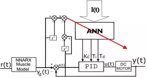
FIGURE 1.
Block diagrams of the muscle emulator. y(t) is the torque output of the DC motor, yd(t) is the output of the muscle model, r(t) is the articular command, and I(t) is the input signals vector based on e(t),e(t-1),e(t-2) and ρ(t) which provides information on the fast variations of r(t).
Walk control approach
This section integrates the muscle emulator into the knee joint control laws. The model of our biped robot consisted of six active degrees of freedom within each leg. Each knee is driven using a 90‐W DC motor (Maxon RE‐35) with 1/90 gear. The biped robot is simulated using the Open Architecture Humanoid Robotics Platform (OpenHRP) simulator. The muscle emulator is implemented to control the DC motor in the low‐level control mode without altering the high‐level robot controls. The high‐level controls include a walking algorithm based on a state machine that provides a stable 3D dynamic biped walk. The walking algorithm and muscle emulator are coded using C++ in the OpenHRP simulator.
CONTROL LEVELS DESCRIPTION
The proposed robot actuator control diagram consists of two levels. The low‐level control is designated by the PID controller. The high‐level control is designated by the dynamic walking algorithm, which tunes the PD controllers and imposes the reference signals following the walking phases (Figure 2).
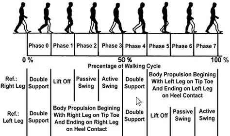
FIGURE 2.
Full human walking cycle (ref. right leg).
Two possibilities exist for the lower level, which are based on using the fixed PID gains for the 12 motors (gains are calculated to have the same adjustments as the real robot) or using the fixed PID gains for all motors except those in the knees, for which PID gains are adapted using the muscle emulator (Figure 3).
The high‐level control adapts the walking PD controller parameters to each walking phase and introduces the corresponding reference signal to the low‐level loop. Note that all of the motors in the low level are driven by PID controllers with desired articular angles.
A general equation of each actuator input Y_d PD controller is given by:

where τ(t) is the desired torque, θd is the desired angle, θ˙dθ˙d is the desired velocity, “Leg” corresponds to the stance or swing leg, and “Phase” corresponds to one of the eight phases of the human walking cycle presented in Figure 3 and “Actuator” corresponds to the hip, knee, and ankle. The values of Kc, and Kdchange during each phase of the walk, as determined by an empirical method when the swing leg approaches the ground [40].
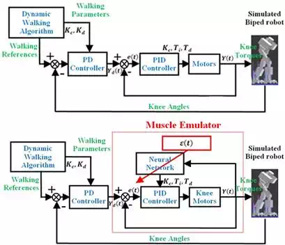
FIGURE 3.
Proposed dynamic walk control diagram. Top: all articular control loop with fixed PID gains Kc, Ti, Td. Bottom: knee adaptive control loop with muscle‐like control loop.
DYNAMIC WALKING ALGORITHM
The proposed walking control approach is based on a sequential analysis of the human walking cycle, the properties of which have been previously determined. This cycle can be divided in eight phases, with one leg acting first as a swing leg and then as a stance leg (Figure 3). Phase 0 is the double support (DS) phase, during which the two legs are touching the ground. Phase 1 is the lift‐off phase, in which hip muscle contractions accelerate the swing leg. Phase 2 is the passive swing, which begins when the thigh is sufficiently accelerated. Phase 3 is the active swing phase. Phase 4 is the DS phase in the next half of the walking cycle. The swing leg assumes the role of the stance leg (ST) in phase 5. Phases 6 and 7 are similar to the fifth phase in terms of functionality related to the stance leg.
We analyzed the human walking cycle and determined that a robot’s dynamic walk can be modeled using a Petri net algorithm (Figure 4). The cycle is divided into 12 states. States 1, 3, 4, 5, 6, and 10 correspond to the swing leg and states 2, 7, 8, 9, and 11 correspond to the stance leg. The initial position is defined when the two legs are in contact with ground (DS) and the robot is standing, but one of the legs is behind the other. All of the transitions in this state machine are defined based on the extreme values of essential leg angles in sagittal or frontal planes. All of the articulations are driven by PD controllers (Eq. (1)), for which each gain changes based on the corresponding phase of the Petri net algorithm. Finally, we can control the robot’s velocity with respect to its body inclination.
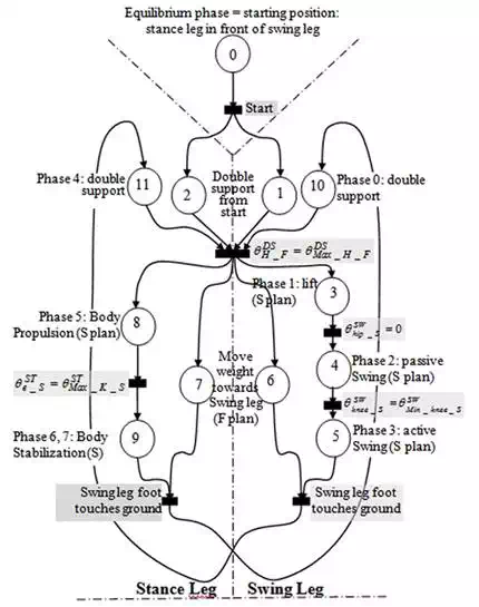
FIGURE 4.
Petri net algorithm for a ROBIAN dynamic walk (S_Plane is sagittal Figure 5. plane, F_Plane is frontal plane).
To stop the robot walking cycle and keep it in a standup stable position, an extension of the Petri net Figure 4 is applied to change our algorithm to introduce a stop phase (Figure 5). The change will start working after swing leg touches ground (State 9, Figure 4, or phases 3 or 7 in Figure 3). We controlled the hip motors to maintain the body in vertical position. By controlling stance and swing leg, the robot will be in stable standup position where we keep little distance between right and left legs foot. From this position we can control the robot to walk again by simple walking algorithm by reapplying our walking Petri net algorithm.
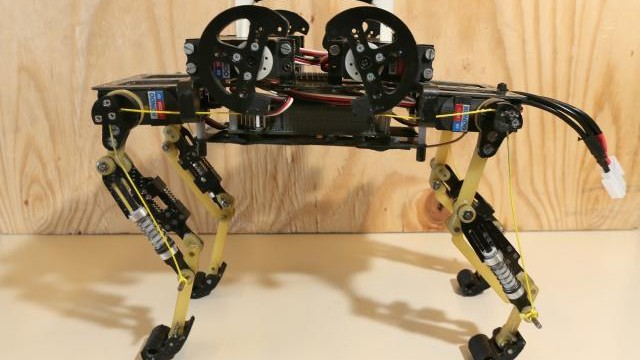
We applied the overall Petri net algorithm using a simulated model of our ROBIAN biped robot (Figure 6). The OpenHRP (Open Architecture Humanoid Robotics Platform) simulator was used, which is a dynamic humanoid robot simulation platform that was developed by AIST, the University of Tokyo, and MSTC. The robot model is programmed in VRML. All of the robot specifications were taken into account. Many control algorithms were tested on the real robot and on the simulated model to improve the similarity.
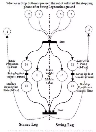
FIGURE 5.
Petri net algorithm for a ROBIAN stop walk.
In the simulations, the walk begins from an initial position where the two feet are touching the ground. The swing leg is behind the stance leg (double support) and the walking speed is 0.65 m/s. The step length and walking speed are controlled by varying the four reference angles. The duration of one complete walking cycle is approximately 1 s. The proposed approach allows us to achieve dynamic ROBIAN walking that is similar to human walking. Simulations show that the walk is stable on a long distance, that is, more than 10 walking cycle. Moreover, the approach also controls the robot’s walk‐standup‐walk cycle, including transitions and stops in a stable limit cycle.
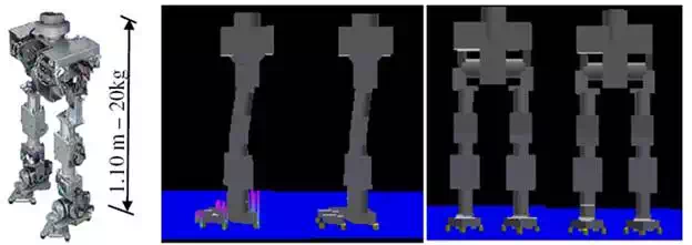
FIGURE 6.
Modeling ROBIAN using OpenHRP.
Nevertheless, the adjustment of PID gains depending on the corresponding phase of the walk algorithm is not sufficient enough to have fluidity in the walk and to adapt the walking gait especially when the robot is unbalanced due to unexpected external forces. It has been seen in introduction that mixing damping joint and damping controller increases the balance. Moreover, the muscle emulator presented in Figure 1 acts simultaneously like a damping joint and a damping controller avoiding any mechanical changes in the robot y. The next section shows that implementation of this muscle emulator in the legs greatly improves the fluidity and stability of the walking algorithm (Figures 4 and 5) against external perturbation and reduces significantly the total power consumption of the robot.
Implementation of the muscle model and comparative results
This section implements the muscle emulator in the walking algorithm presented in the previous section. Only the knee joints are modified to not complicate the algorithm. The simulation results are compared with those obtained without the muscle model.
CONTINUOUS WALKING GAIT
The results presented in Figure 7 illustrate that the robot’s articular angles are close to those of humans and that trajectories generated with the muscle emulator are closer than those simulated without it. Stance phase ankle motions are significantly improved. However, the difference between the robot and human ankle angles remains the same in the swing phase, and the robot’s foot control is dissimilar to a human foot in the landing phase. This is because the human foot exhibits significant flexibility compared to the rigid robot foot. This assumption has been confirmed by several experiments conducted by medical teams (Dr. B. Bussel and Dr. D. Pradon of the APHP Poincaré Hospital, Garches, France). These experiments recorded and compared human walking gaits based on rigid and non‐rigid human foot soles. Figure 8 depicts the hip, knee, and ankle during one of these experiments. The results show that the rigid sole changes the other articulation movements, especially those in the ankle, in which the extension movement is significantly reduced.
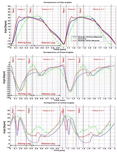
FIGURE 7.
Comparison of the joint angles between an average 13‐year‐old and ROBIAN (right leg) over two walking cycles for the hip, knee, and ankle. The phases correspond to the human phases in Figure 3. The speed is 0.6 m/s.
The robot foot then lands parallel to ground and the swinging leg foot begins the swing phase. In the passive swing phase, ankle motors were controlled to keep the foot parallel to the ground. The foot was stabilized in this position in the active swing phase, allowing the foot to hit the ground in a manner that distributed the ground reaction forces equally throughout the foot.
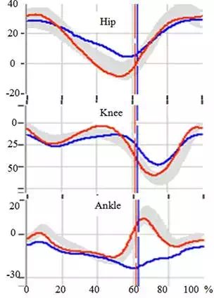
FIGURE 8.
Comparison of the articular angles (in degrees) of the hip (flexion/extension), knee, and ankle (plantarflexion/dorsiflexion) in humans, with a rigid and non‐rigid human foot soles. Time is expressed as a percentage of the human walk cycle duration. The experiments were conducted by Dr. D. Pradon and Dr. B. Bussel of the APHP R. Poincaré Hospital, Garches, France.
Figure 9 compares the articular joint power consumptions in the three articulations for one walking cycle with and without the muscle emulator in the knees. One can see that the muscle emulator reduces the power consumed at each articulation, even if it is only implemented in the knees. Other simulations illustrate that the emulator reduces the working duration of the DC motor in the overload zone defined by the constructor.
Figure 10 depicts the phase plane of three joint angles over 10 walking cycles with and without a muscle emulator in the knees. The muscle emulator induces changes in each articular movement, especially in the knees, for which the amplitude or flexion/extension is reduced and the extension reaches 0°. The convergence of the trajectories between the transient and stable walking cycles illustrates the stability of the walk.
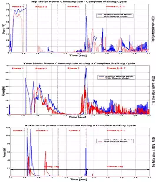
FIGURE 9.
Comparison of the joint power consumption (right leg) of the hip, knee and ankle of ROBIAN over one walking cycles with and without a muscle emulator. The speed is 0.6 m/s.
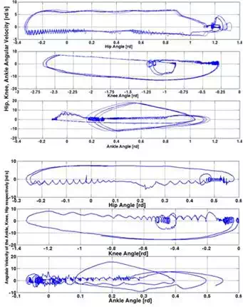
FIGURE 10.
Phase plan of the three joints for 10 walking cycles. Top: without the muscle emulator. Bottom: with the muscle emulator.
WALK‐HALT‐WALK TRANSITIONS
Figure 11 presents the different angular variations of both legs during a walk‐halt‐walk cycle that takes approximately 15 s. The curves show the differences between the two models during walking and stop processes. When walking, the curves are nearly identical, suggesting that the emulator does not change the robot’s velocity. However, it is clear that the cycle induced with the muscle emulator displays more reduction than the simulation without the emulator. In addition, the emulator allows the robot to stop in a stand‐up position with legs extended (hip and knee angles close to zero). The speed oscillations observed during the stop, which are reduced by the emulator, are due to the balance control instabilities, especially in the ankles. The muscle emulator acts as a low‐frequency pass filter.
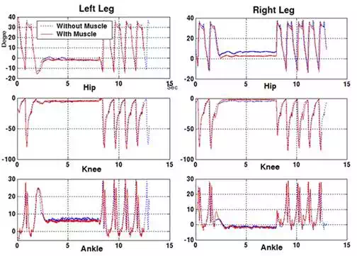
FIGURE 11.
Angular variations of the hips, knees, and ankles of ROBIAN during a complete “walk‐halt‐walk” cycle (2 s of walking, 6 s of stopping and 8 s of walking).
Figure 12 shows the robot’s trunk speed variations, which correspond to the curves in Figure 10. Transitions occur between the walking and stopping and stopping and walking processes. During these transitions, the balance of the robot is controlled based on the states and transitions of the Petri net. The shapes are nearly identical. However, the transient speed at the beginning of the stop is slightly amortized with the muscle.
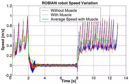
FIGURE 12.
Trunk speed during a complete walk‐stop‐walk cycle.
STABILITY VERSUS EXTERNAL PERTURBATION FORCES
We simulated the external forces that affect the robot in the sagittal and frontal planes to assess the robustness of the walking algorithm with the muscle emulator. Figure 13 shows the instantaneous sagittal plane horizontal velocity variation due to a 35 N and 100 ms thrust force applied forward and a 50 N force (100 ms duration) applied backward. Note that the speed of the robot initially decreases. The velocity then maintains the same average speed with muscle emulator, but a larger average speed without. This suggests that the robot is close to falling after being pushed without the muscle emulator.
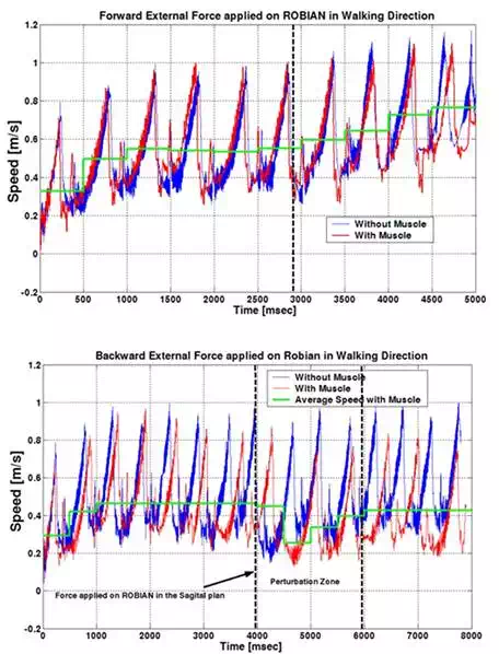
FIGURE 13.
Trunk speed of ROBIAN in the sagittal plane, after applying a force. Top: in the direction of the walk. Bottom: in the direction opposite the walk.
Figure 14 shows the effect on the instantaneous frontal plane horizontal velocity due to a 120 N and 100 ms thrust force applied in the direction perpendicular to the walking robot. Note that movement of the robot in the plane is less than for the case with the emulator. It is clear that the stability of the robot is improved by the emulator, as the displacement of the robot is much smaller compared to the results without the emulator. The emulator allows the robot to withstand a 30% larger force than the simulation without the emulator. In fact, the robot falls when the same force is applied without the emulator.
Although the simulations with the emulator indicate that the robot can withstand a 30% larger applied force than those without the emulator, a sufficiently large sagittal plane force (approximately 85 N for 100 ms forward or 65 N backward) cannot be counteracted, and the robot falls in the direction of the force.
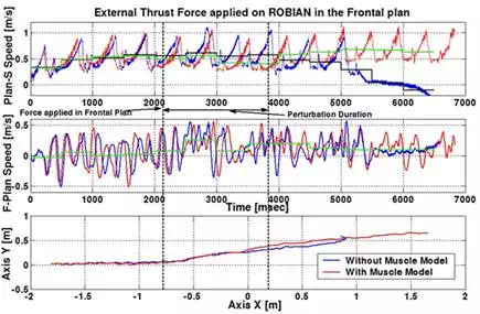
FIGURE 14.
Trunk speed of ROBIAN (in sagittal plane) and trunk position (in the frontal plane), after applying a thrust force perpendicular to the direction of walking (frontal plane).
Conclusion
The contribution of this chapter is to compare and analyze the effects a muscle emulator on the walking efficiency of a biped robot. The results indicate that the use of a muscle emulator in the DC motor control loops of humanoid robots provides a compliance property in articular joints. Thus, the walking performance is improved, as follows:
● the muscle emulator significantly reduced the total power consumption.
● the work required by the electric motors decreased, and the motors work less in the authorized overload zone.
● the equilibrium of the robot can withstand 25–30% larger external forces with the muscle emulator.
● the algorithm allows the robot to stand with the knees fully extended in the stop position.
This model benefits from the advantages and simplicity of electric motor implementation, as well as from the benefits of human muscle compliance, which allow for dynamic walking without adding a physical element to the robot.