
One of the central issues in robotics and animal motor control is the problem of trajectory generation and modulation. Since in many cases trajectories have to be modified on-line when goals are changed, obstacles are encountered, or when external perturbations occur, the notions of trajectory generation and trajectory modulation are tightly coupled.
This chapter addresses some of the issues related to trajectory generation and modulation, including the supervised learning of periodic trajectories, and with an emphasis on the learning of the frequency and achieving and maintaining synchronization to external signals. Other addressed issues include robust movement execution despite external perturbations, modulation of the trajectory to reuse it under modified conditions and adaptation of the learned trajectory based on measured force information. Different experimental scenarios on various robotic platforms are described.
For the learning of a periodic trajectory without specifying the period and without using traditional off-line signal processing methods, our approach suggests splitting the task into two sub-tasks: (1) frequency extraction, and (2) the supervised learning of the waveform. This is done using two ingredients: nonlinear oscillators, also combined with an adaptive Fourier waveform for the frequency adaptation, and nonparametric regression 1 techniques for shaping the attractor landscapes according to the demonstrated trajectories. The systems are designed such that after having learned the trajectory, simple changes of parameters allow modulations in terms of, for instance, frequency, amplitude and oscillation offset, while keeping the general features of the original trajectory, or maintaining synchronization with an external signal.
![]() The system we propose in this paper is based on the motion imitation approach described in (Ijspeert et al., 2002; Schaal et al., 2007). That approach uses two dynamical systems like the system presented here, but with a simple nonlinear oscillator to generate the phase and the amplitude of the periodic movements. A major drawback of that approach is that it requires the frequency of the demonstration signal to be explicitly specified. This means that the frequency has to be either known or extracted from the recorded signal by signal
The system we propose in this paper is based on the motion imitation approach described in (Ijspeert et al., 2002; Schaal et al., 2007). That approach uses two dynamical systems like the system presented here, but with a simple nonlinear oscillator to generate the phase and the amplitude of the periodic movements. A major drawback of that approach is that it requires the frequency of the demonstration signal to be explicitly specified. This means that the frequency has to be either known or extracted from the recorded signal by signal
1 The term “nonparametric” is to indicate that the data to be modeled stem from very large families of distributions which cannot be indexed by a finite dimensional parameter vector in a natural way. It does not mean that there are no parameters.processing methods, e.g. Fourier analysis. The main difference of our new approach is that we use an adaptive frequency oscillator (Buchli & Ijspeert, 2004; Righetti & Ijspeert,2006), which has the process of frequency extraction and adaptation totally embedded into its dynamics. The frequency does not need to be known or extracted, nor do we need to perform any transformations (Righetti et al., 2006). This simplifies the process of teaching a new task/trajectory to the robot. Additionally, the system can work incrementally in on-line settings. We use two different approaches. One uses several frequency oscillators to approximate the input signal, and thus demands a logical algorithm to extract the basic frequency of the input signal. The other uses only one oscillator and higher harmonics of the extracted frequency. It also includes an adaptive fourier series.
Our approach is loosely inspired from dynamical systems observed in vertebrate central nervous systems, in particular central pattern generators (Ijspeert, 2008a). Additionally, our work fits in the view that biological movements are constructed out of the combination of “motor primitives” (Mataric, 1998; Schaal, 1999), and the system we develop could be used as blocks or motor primitives for generating more complex trajectories.
Overview of the research field
One of the most notable advantages of the proposed system is the ability to synchronize with an external signal, which can effectively be used in control of rhythmic periodic task where the dynamic behavior and response of the actuated device are critical. Such robotic tasks include swinging of different pendulums (Furuta, 2003; Spong, 1995), playing with different toys, i.e. the yo-yo (Hashimoto & Noritsugu, 1996; Jin et al., 2009; Jin & Zacksenhouse, 2003; Žlajpah, 2006) or a gyroscopic device called the Powerball (Cafuta & Curk, 2008; Gams et al., 2007; Heyda, 2002; Petricˇ et al., 2010), juggling (Buehler et al., 1994; Ronsse et al., 2007; Schaal & Atkeson, 1993; Williamson, 1999) and locomotion (Ijspeert, 2008b; Ilg et al., 1999; Morimoto et al., 2008). Rhythmic tasks are also handshaking (Jindai & Watanabe, 2007; Kasuga & Hashimoto, 2005; Sato et al., 2007) and even handwriting (Gangadhar et al., 2007; Hollerbach,1981). Performing these tasks with robots requires appropriate trajectory generation and foremost precise frequency tuning by determining the basic frequency. We denote the lowest frequency relevant for performing a given task, with the term “basic frequency”.
Different approaches that adjust the rhythm and behavior of the robot, in order to achieve synchronization, have been proposed in the past. For example, a feedback loop that locks onto the phase of the incoming signal. Closed-loop model-based control (An et al., 1988), as a very common control of robotic systems, was applied for juggling (Buehler et al., 1994; Schaal
& Atkeson, 1993), playing the yo-yo (Jin & Zackenhouse, 2002; Žlajpah, 2006) and also for the control of quadruped (Fukuoka et al., 2003) and in biped locomotion (Sentis et al., 2010; Spong & Bullo, 2005). Here the basic strategy is to plan a reference trajectory for the robot, which is based on the dynamic behavior of the actuated device. Standard methods for reference trajectory tracking often assume that a correct and exhaustive dynamic model of the object is available (Jin & Zackenhouse, 2002), and their performance may degrade substantially if the accuracy of the model is poor.
An alternative approach to controlling rhythmic tasks is with the use of nonlinear oscillators. Oscillators and systems of coupled oscillators are known as powerful modeling tools (Pikovsky et al., 2002) and are widely used in physics and biology to model phenomena as diverse as neuronal signalling, circadian rhythms (Strogatz, 1986), inter-limb coordination (Haken et al., 1985), heart beating (Mirollo et al., 1990), etc. Their properties, which include robust limit cycle behavior, online frequency adaptation (Williamson, 1998) and self-sustained limit cycle generation on the absence of cyclic input (Bailey, 2004), to name just a few, make them suitable for controlling rhythmic tasks.
Different kinds of oscillators exist and have been used for control of robotic tasks. The van der Pol non-linear oscillator (van der Pol, 1934) has successfully been used for skill entrainment on a swinging robot (Veskos & Demiris, 2005) or gait generation using coupled oscillator circuits, e.g. (Jalics et al., 1997; Liu et al., 2009; Tsuda et al., 2007). Gait generation has also been studied using the Rayleigh oscillator (Filho et al., 2005). Among the extensively used oscillators is also the Matsuoka neural oscillator (Matsuoka, 1985), which models two mutually inhibiting neurons. Publications by Williamson (Williamson, 1999; 1998) show the use of the Matsuoka oscillator for different rhythmic tasks, such as resonance tuning, crank turning and playing the slinky toy. Other robotic tasks using the Matsuoka oscillator include control of giant swing problem (Matsuoka et al., 2005), dish spinning (Matsuoka & Ooshima, 2007) and gait generation in combination with central pattern generators (CPGs) and phase-locked loops (Inoue et al., 2004; Kimura et al., 1999; Kun & Miller, 1996).
On-line frequency adaptation, as one of the properties of non-linear oscillators (Williamson, 1998) is a viable alternative to signal processing methods, such as fast Fourier transform (FFT), for determining the basic frequency of the task. On the other hand, when there is no input into the oscillator, it will oscillate at its own frequency (Bailey, 2004). Righetti et al. have introduced adaptive frequency oscillators (Righetti et al., 2006), which preserve the learned frequency even if the input signal has been cut. The authors modify non-linear oscillators or pseudo-oscillators with a learning rule, which allows the modified oscillators to learn the frequency of the input signal. The approach works for different oscillators, from a simple phase oscillator (Gams et al., 2009), the Hopf oscillator, the Fitzhugh-Nagumo oscillator, etc. (Righetti et al., 2006). Combining several adaptive frequency oscillators in a feedback loop allows extraction of several frequency components (Buchli et al., 2008; Gams et al., 2009). Applications vary from bipedal walking (Righetti & Ijspeert, 2006) to frequency tuning of a hopping robot (Buchli et al., 2005). Such feedback structures can be used as a whole imitation system that both extracts the frequency and learns the waveform of the input signal.
Not many approaches exist that combine both frequency extraction and waveform learning in imitation systems (Gams et al., 2009; Ijspeert, 2008b). One of them is a two-layered imitation system, which can be used for extracting the frequency of the input signal in the first layer and learning its waveform in the second layer, which is the basis for this chapter. Separate frequency extraction and waveform learning have advantages, since it is possible to independently modulate temporal and spatial features, e.g. phase modulation, amplitude modulation, etc. Additionally a complex waveform can be anchored to the input signal. Compact waveform encoding, such as splines (Miyamoto et al., 1996; Thompson & Patel,1987; Ude et al., 2000), dynamic movement primitives (DMP) (Schaal et al., 2007), or Gaussian mixture models (GMM) (Calinon et al., 2007), reduce computational complexity of the process. In the next sections we first give details on the two-layered movement imitation system and then give the properties. Finally, we propose possible applications.
Two-layered movement imitation system
In this chapter we give details and properties of both sub-systems that make the two-layered movement imitation system . We also give alternative possibilities for the canonical dynamical system
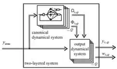
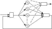
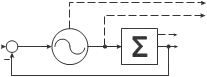
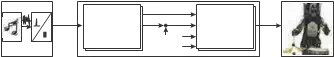
Fig. 1. Proposed structure of the system. The two-layered system is composed of the Canonical Dynamical System as the first layer for the frequency adaptation, and the Output Dynamical System for the learning as the second layer. The input signal ydemo (t) is an arbitrary Q-dimensional periodic signal. The Canonical Dynamical System outputs the fundamental frequency Ω and phase of the oscillator at that frequency, Φ, for each of the Q DOF, and the Output Dynamical System learns the waveform.
Figure 1 shows the structure of the proposed system for the learning of the frequency and the waveform of the input signal. The input into the system ydemo (t) is an arbitrary periodic signal of one or more degrees of freedom (DOF).
The task of frequency and waveform learning is split into two separate tasks, each performed by a separate dynamical system. The frequency adaptation is performed by the Canonical Dynamical System, which either consists of several adaptive frequency oscillators in a feedback structure, or a single oscillator with an adaptive Fourier series. Its purpose is to extract the basic frequency Ω of the input signal, and to provide the phase Φ of the signal at this frequency.
These quantities are fed into the Output Dynamical System, whose goal is to adapt the shape of the limit cycle of the Canonical Dynamical System, and to learn the waveform of the input signal. The resulting output signal of the Output Dynamical System is not explicitly encoded but generated during the time evolution of the Canonical Dynamical System, by using a set of weights learned by Incremental Locally Weighted Regression (ILWR) (Schaal & Atkeson,1998).
Both frequency adaptation and waveform learning work in parallel, thus accelerating the process. The output of the combined system can be, for example, joint coordinates of the robot, position in task space, joint torques, etc., depending on what the input signal represents.
In the next section we first explain the second layer of the system – the output dynamical system – which learns the waveform of the input periodic signal once the frequency is determined.
Output dynamical system
The output dynamical system is used to learn the waveform of the input signal. The explanation is for a 1 DOF signal. For multiple DOF, the algorithm works in parallel for all the degrees of freedom.
The following dynamics specify the attractor landscape of a trajectory y towards the anchor point g, with the Canonical Dynamical System providing the phase Φ to the function Ψi of the control policy:
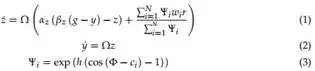
Here Ω (chosen amongst the ωi ) is the frequency given by canonical dynamical system, Eq. (10), αZ and βz are positive constants, set to αz = 8 and βz = 2 for all the results; the ratio 4:1 ensures critical damping so that the system monotonically varies to the trajectory oscillating
around g – an anchor point for the oscillatory trajectory. N is the number of Gaussian-like periodic kernel functions Ψi , which are given by Eq. (3). wi is the learned weight parameter and r is the amplitude control parameter, maintaining the amplitude of the demonstration signal with r = 1. The system given by Eq. (1) without the nonlinear term is a second-order linear system with a unique globally stable point attractor (Ijspeert et al., 2002). But, because of the periodic nonlinear term, this system produces stable periodic trajectories whose frequency is Ω and whose waveform is determined by the weight parameters wi . In Eq. (3), which determines the Gaussian-like kernel functions Ψi , h determines their width, which is set to h = 2.5N for all the results presented in the paper unless stated otherwise, and ci are equally spaced between 0 and 2π in N steps.
As the input into the learning algorithm we use triplets of position, velocity and acceleration ydemo (t), y˙ demo (t), and y¨demo (t) with demo marking the input or demonstration trajectory we are trying to learn. With this Eq. (1) can be rewritten as
1
Ω z˙ − αz (βz (g − y) − z) =
| i=1 |
∑N Ψi wi r
| N |
∑i=1 Ψi
(4)
Locally weighted regression corresponds to finding, for each kernel function Ψi , the weight vector wi , which minimizes the quadratic error criterion 2
P
Ji = ∑ Ψi (t) ftarg (t) − wi r(t)
t=1
(5)
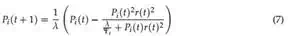
![]() where t is an index corresponding to discrete time steps (of the integration). The regression can be performed as a batch regression, or alternatively, we can perform the minimization of the Ji cost function incrementally, while the target data points ftarg (t) arrive. As we want continuous learning of the demonstration signal, we use the latter. Incremental regression is done with the use of recursive least squares with a forgetting factor of λ, to determine the parameters (or weights) wi . Given the target data ftarg (t) and r(t), wi is updated by
where t is an index corresponding to discrete time steps (of the integration). The regression can be performed as a batch regression, or alternatively, we can perform the minimization of the Ji cost function incrementally, while the target data points ftarg (t) arrive. As we want continuous learning of the demonstration signal, we use the latter. Incremental regression is done with the use of recursive least squares with a forgetting factor of λ, to determine the parameters (or weights) wi . Given the target data ftarg (t) and r(t), wi is updated by
wi (t + 1) = wi (t)+ Ψi Pi (t + 1)r(t)er (t) (6)
2 LWR is derived from a piecewise linear function approximation approach (Schaal & Atkeson, 1998), which decouples a nonlinear least-squares learning problem into several locally linear learning problems, each characterized by the local cost function Ji . These local problems can be solved with standard weighted least squares approaches.
![]()
![]() 2 400
2 400
1 200
![]()
![]() 0 0
0 0
−1 −200
−2
10 10.5 11 11.5 12
−400
10 10.5 11 11.5 12
![]()
![]() 20 1
20 1
10
![]()
![]() 0 0.5
0 0.5
−10
−20
10 10.5 11 11.5 12
![]() 2
2
1.5
![]() 1
1
0.5
![]() 0
0
10 10.5 11 11.5 12
![]()
![]() 6
6
4
2
0.6
0.4
0.2
0
N = 10
N = 25
 N = 50
0
10 10.5 11 11.5 12
t [s]
0
10 10.5 11 11.5 12
t [s]
−0.2
20 20.2 20.4 20.6 20.8 21 21.2 21.4 21.6 21.8 22
t [s]
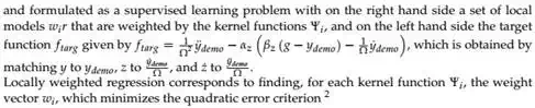
Fig. 2. Left: The result of Output Dynamical System with a constant frequency input and with continuous learning of the weights. In all the plots the input signal is the dash-dot line while the learned signal is the solid line. In the middle-right plot we can see the evolution of the kernel functions. The kernel functions are a function of Φ and do not necessarily change uniformly (see also Fig. 7). In the bottom right plot the phase of the oscillator is shown. The amplitude is here r = 1, as shown bottom-left. Right: The error of learning decreases with the increase of the number of Gaussian-like kernel functions. The error, which is quite small, is mainly due to a very slight (one or two sample times) delay of the learned signal.
er (t) = ftarg (t) − wi (t)r(t).
(8) P, in general, is the inverse covariance matrix (Ljung & Söderström, 1986). The recursion is started with wi = 0 and Pi = 1. Batch and incremental learning regressions provide identical weights wi for the same training sets when the forgetting factor λ is set to one. Differences appear when the forgetting factor is less than one, in which case the incremental regression
gives more weight to recent data (i.e. tends to forget older ones). The error of weight learning er (Eq. (8)) is not “related” to e when extracting frequency components (Eq. (11)). This allows for complete separation of frequency adaptation and waveform learning.
Figure 2 left shows the time evolution of the Output Dynamical System anchored to a Canonical Dynamical System with the frequency set at Ω = 2π rad/s, and the weight parameters wi adjusted to fit the trajectory ydemo (t) = sin (2πt) + cos (4πt) + 0.4sin(6πt). As
we can see in the top-left plot, the input signal and the reconstructed signal match closely. The matching between the reconstructed signal and the input signal can be improved by increasing the number of Gaussian-like functions.
Parameters of the Output Dynamical System
When tuning the parameters of the Output Dynamical System, we have to determine the number of Gaussian-like Kernel functions N, and specially the forgetting factor λ. The number N of Gaussian-like kernel functions could be set automatically if we used the locally weighted learning (Schaal & Atkeson, 1998), but for simplicity it was here set by hand. Increasing the number increases the accuracy of the reconstructed signal, but at the same time also increases the computational cost. Note that LWR does not suffer from problems of overfitting when the number of kernel functions is increased.3 Figure 2 right shows the error of learning er when using N = 10, N = 25, and N = 50 on a signal ydemo (t) = 0.65sin (2πt) + 1.5cos (4πt) + 0.3sin (6πt). Throughout the paper, unless specified otherwise, N = 25.
The forgetting factor λ ∈ [0, 1] plays a key role in the behavior of the system. If it is set high, the system never forgets any input values and learns an average of the waveform over multiple periods. If it is set too low, it forgets all, basically training all the weights to the last value. We set it to λ = 0.995.
Canonical dynamical system
The task of the Canonical Dynamical System is two-fold. Firstly, it has to extract the fundamental frequency Ω of the input signal, and secondly, it has to exhibit stable limit cycle behavior in order to provide a phase signal Φ, that is used to anchor the waveform of the output signal. Two approaches are possible, either with a pool of oscillators (PO), or with an adaptive Fourier Series (AF).
Using a pool of oscillators
As the basis of our canonical dynamical system we use a set of phase oscillators, see e.g. (Buchli et al., 2006), to which we apply the adaptive frequency learning rule as introduced in (Buchli & Ijspeert, 2004) and (Righetti & Ijspeert, 2006), and combine it with a feedback structure (Righetti et al., 2006) shown in Figure 3. The basic idea of the structure is that each of the oscillators will adapt its frequency to one of the frequency components of the input signal, essentially “populating” the frequency spectrum.
We use several oscillators, but are interested only in the fundamental or lowest non-zero frequency of the input signal, denoted by Ω, and the phase of the oscillator at this frequency, denoted by Φ. Therefore the feedback structure is followed by a small logical block, which chooses the correct, lowest non-zero, frequency. Determining Ω and Φ is important because with them we can formulate a supervised learning problem in the second stage – the Output Dynamical System, and learn the waveform of the full period of the input signal.
ydemo
+
 ω1(t),ɸ1
ω2(t),ɸ2
| e |
ω3(t),ɸ3
lowest non-zero
Ω,Φ
– Σαicos(ɸi)
y^
ωM(t),ɸM
Fig. 3. Feedback structure of a network of adaptive frequency phase oscillators, that form the Canonical Dynamical System. All oscillators receive the same input and have to be at different starting frequencies to converge to different final frequencies. Refer also to text and Eqs. (9-13).
![]() The feedback structure of M adaptive frequency phase oscillators is governed by the following equations:
The feedback structure of M adaptive frequency phase oscillators is governed by the following equations:
3 This property is due to solving the bias-variance dilemma of function approximation locally with a closed form solution to leave-one-out cross-validation (Schaal & Atkeson, 1998).
φ˙ i = ωi − Ke sin(φi ) (9)
ω˙ i = −Ke sin(φi ) (10)
e = ydemo − yˆ
M
(11)
yˆ = ∑ αi cos(φi ) (12)
i=1
α˙ i = η cos(φi )e (13)
where K is the coupling strength, φi is the phase of oscillator i, e is the input into the oscillators, ydemo is the input signal, yˆ is the weighted sum of the oscillators’ outputs, M is the number of oscillators, αi is the amplitude associated to the i-th oscillator, and η is a learning constant. In the experiments we use K = 20 and η = 1, unless specified otherwise.
Eq. (9) and (10) present the core of the Canonical Dynamical System – the adaptive frequency phase oscillator. Several (M) such oscillators are used in a feedback loop to extract separate frequency components. Eq. (11) and (12) specify the feedback loop, which needs also amplitude adaptation for each of the frequency components (Eq. (13)).
As we can see in Figure 3, each of the oscillators of the structure receives the same input signal, which is the difference between the signal to be learned and the signal already learned by the feedback loop, as in Eq. (11). Since a negative feedback loop is used, this difference approaches zero as the weighted sum of separate frequency components, Eq. (12), approaches the learned signal, and therefore the frequencies of the oscillators stabilize. Eq. (13) ensures amplitude adaptation and thus the stabilization of the learned frequency. Such a feedback structure performs a kind of dynamic Fourier analysis. It can learn several frequency components of the input signal (Righetti et al., 2006) and enables the frequency of a given oscillator to converge as t → ∞, because once the frequency of a separate oscillator is set, it is deducted from the demonstration signal ydemo , and disappears from e (due to the negative feedback loop). Other oscillators can thus adapt to other remaining frequency components. The populating of the frequency spectrum is therefore done without any signal processing, as the whole process of frequency extraction and adaptation is totally embedded into the dynamics of the adaptive
frequency oscillators.
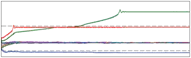
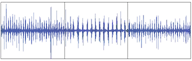
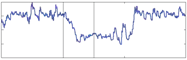
Frequency adaptation results for a time-varying signal are illustrated in Figure 4, left. The top plot shows the input signal ydemo , the middle plot the extracted frequencies, and the bottom plot the error of frequency adaptation. The figure shows results for both approaches, using a pool of oscillators (PO) and for using one oscillator and an adaptive Fourier series (AF), explained in the next section. The signal itself is of three parts, a non-stationary signal (presented by a chirp signal), followed by a step change in the frequency of the signal, and
in the end a stationary signal. We can see that the output frequency stabilizes very quickly at the (changing) target frequency. In general the speed of convergence depends on the coupling strength K (Righetti et al., 2006). Besides the use for non-stationary signals, such as chirp signals, coping with the change in frequency of the input signal proves especially useful when adapting to the frequency of hand-generated signals, which are never stationary. In this particular example, a single adaptive frequency oscillator in a feedback loop was enough, because the input signal was purely sinusoidal.
The number of adaptive frequency oscillators in a feedback loop is therefore a matter of design. There should be enough oscillators to avoid missing the fundamental frequency and to limit the variation of frequencies described below when the input signal has many
![]() 40
40
20
0
1
![]() 0
0 
−1
 20 ωt ΩAF ΩPO
15
![]() 10
10
5
8

![]() 6
6
0 100 200 300 400 500

 0.5
0.5
![]() 0
0

![]() −0.5
−0.5
![]() 200
200


| 01020304050602020.5 21 150 150.5 151 350 350.5 351 t [s] t [s] |
0
0.04
![]()


 0
0
Fig. 4. Left: Typical convergence of an adaptive frequency oscillator combined with an adaptive Fourier series (-) compared to a system with a poll of i oscillators (-.-). One oscillator is used in both cases. The input is a periodic signal (y = sin(ωt t), with ωt = (6π − π/5t) rad/s for t < 20 s, followed by ωt = 2π rad/s for t < 30 s, followed again by ωt = 5π rad/s for t < 45 s and finally ωt = 3π rad/s). Frequency adaptation is presented in the middle plot, starting at Ω0 = π rad/s, where ωt is given by the dashed line and Ω by the solid line. The square error between the target and the extracted frequency is shown in the bottom plot. We can see that the adaptation is successful for non-stationary signals, step changes and stationary signals. Right: Comparison between using the PO and the AF approaches for the canonical dynamical system. The first plot shows the evolution of frequency distribution using a pool of 10 oscillators. The second plot shows the extracted frequency using the AF approach. The comparison of the target and the approximated signals is presented in the third plot. The thin solid line presents the input signal ydemo , the thick solid line presents the AF approach yˆ and the dotted line presents the PO approach yˆo . The square difference between the input and the approximated signals is presented in the bottom plot.
frequencies components. A high number of oscillators can be used. Beside the almost negligible computational costs, using too many oscillators does not affect the solution. A practical problem that arises is that the oscillators’ frequencies might come too close together, and then lock onto the same frequency component. To solve this we separate their initial frequencies ω0 in a manner that suggests that (preferably only) one oscillator will go for the offset, one will go for the highest frequency, and the others will “stay between”.
With a high number of oscillators, many of them want to lock to the offset (0 Hz). With the target frequency under 1 rad/s the oscillations of the estimated frequency tend to be higher, which results in longer adaptation times. This makes choosing the fundamental frequency
without introducing complex decision-making logic difficult. Results of frequency adaptation for a complex waveform are presented in Fig. 4, where results for both PO and AF approach are presented.
Besides learning, we can also use the system to repeat already learned signals. It this case, we cut feedback to the adaptive frequency oscillators by setting e(t) = 0. This way the oscillators continue to oscillate at the frequency to which they adapted. We are only interested in the fundamental frequency, determined by
Φ˙ = Ω (14)
Ω˙ = 0 (15)
which is derived from Eqs. (9 and 10). This is also the equation of a normal phase oscillator.
Using an adaptive Fourier series
In this section an alternative, novel architecture for the canonical dynamical system is presented. As the basis of the canonical dynamical system one single adaptive frequency phase oscillator is used. It is combined with a feedback structure based on an adaptive Fourier series (AF). The feedback structure is shown in Fig. 5. The feedback structure of an adaptive frequency phase oscillator is governed by
φ˙ = Ω − Ke sin Φ, (16)
Ω˙ = −Ke sin Φ, (17)
e = ydemo − yˆ, (18)
where K is the coupling strength, Φ is the phase of the oscillator, e is the input into the oscillator and ydemo is the input signal. If we compare Eqs. (9, 10) and Eqs. (16, 17), we can see that the basic frequency Ω and the phase Φ are in Eqs. (16, 17) clearly defined and no additional algorithm is required to determine the basic frequency. The feedback loop signal yˆ in (18) is given by the Fourier series
M
yˆ = ∑ (αi cos(iφ)+ βi sin(iφ)), (19)
i=0
and not by the sum of separate frequency components as in Eq. (12). In Eq. (19) M is the number of components of the Fourier series and αi , βi are the amplitudes associated with the Fourier series governed by
| e |
ydemo
α˙ i = η cos(iφ)e, (20)
β˙ i = η sin(iφ)e, (21)
AF
AF
y
Fig. 5. Feedback structure of an adaptive frequency oscillator combined with a dynamic
Fourier series. Note that no logical algorithm is needed.
where η is the learning constant and i = 0…M. As shown in Fig. 5, the oscillator input is the difference between the input signal ydemo and the Fourier series yˆ. Since a negative feedback loop is used, the difference approaches zero when the Fourier series representation yˆ approaches the input signal y. Such a feedback structure performs a kind of adaptive Fourier analysis. Formally, it performs only a Fourier series approximation, because input signals may drift in frequency and phase. General convergence remains an open issue. The number of harmonic frequency components it can extract depends on how many terms of the Fourier series are used.
As it is able to learn different periodic signals, the new architecture of the canonical dynamical system can also be used as an imitation system by itself. Once e is stable (zero), the periodic signal stays encoded in the Fourier series, with an accuracy that depends on the number of elements used in Fourier series. The learning process is embedded and is done in real-time. There is no need for any external optimization process or other learning algorithm.
It is important to point out that the convergence of the frequency adaptation (i.e. the behavior of Ω) should not be confused with locking behavior (Buchli et al., 2008) (i.e. the classic phase locking behavior, or synchronization, as documented in the literature (Pikovsky et al.,
2002)). The frequency adaptation process is an extension of the common oscillator with a fixed intrinsic frequency. First, the adaptation process changes the intrinsic frequency and not only the resulting frequency. Second, the adaptation has an infinite basin of attraction (see (Buchli et al., 2008)), third the frequency stays encoded in the system when the input is removed (e.g. set to zero or e ≈ 0). Our purpose is to show how to apply the approach for control of rhythmic robotic task. For details on analyzing interaction of multiple oscillators see e.g. (Kralemann et al., 2008).
Augmenting the system with an output dynamical system makes it possible to synchronize the movement of the robot to a measurable periodic quantity of the desired task. Namely, the waveform and the frequency of the measured signal are encoded in the Fourier series and the desired robot trajectory is encoded in the output dynamical system. Since the adaptation of the frequency and learning of the desired trajectory can be done simultaneously, all of the system time-delays, e.g. delays in communication, sensor measurements delays, etc., are automatically included. Furthermore, when a predefined motion pattern for the trajectory is used, the phase between the input signal and output signal can be adjusted with a phase lag parameter φl (see Fig. 9). This enables us to either predefine the desired motion or to teach the robot how to preform the desired rhythmic task online.
Even though the canonical dynamical system by itself can reproduce the demonstration signal, using the output dynamical system allows for easier modulation in both amplitude and frequency, learning of complex patterns without extracting all frequency components and acts as a sort of a filter. Moreover, when multiple output signals are needed, only one canonical system can be used with several output systems which assure that the waveforms of the different degrees-of-freedom are realized appropriately.
On-line learning and modulation
On-line modulations
The output dynamical system allows easy modulation of amplitude, frequency and center of oscillations. Once the robot is performing the learned trajectory, we can change all of these by changing just one parameter for each. The system is designed to permit on-line modulations of the originally learned trajectories. This is one of the important motivations behind the use of dynamical systems to encode trajectories.
Changing the parameter g corresponds to a modulation of the baseline of the rhythmic movement. This will smoothly shift the oscillation without modifying the signal shape. The results are presented in the second plot in Figure 6 left. Modifying Ω and r corresponds to the changing of the frequency and the amplitude of the oscillations, respectively. Since our differential equations are of second order, these abrupt changes of parameters result in smooth variations of the trajectory y. This is particularly useful when controlling articulated robots, which require trajectories with limited jerks. Changing of the parameter Ω only comes into consideration when one wants to repeat the learned signal at a desired frequency that is different from the one we adapted to with our Canonical Dynamical System. Results of changing the frequency Ω are presented in the third plot of Figure 6 left. Results of modulating the amplitude parameter r are presented in the bottom plot of Figure 6 left.
Perturbations and modified feedback
Dealing with perturbations
The Output Dynamical System is inherently robust against perturbations. Figure 6 right illustrates the time evolution of the system repeating a learned trajectory at the frequency of 1 Hz, when the state variables y, z and Φ are randomly changed at time t = 30 s. From the results we can see that the output of the system reverts smoothly to the learned trajectory. This is an important feature of the approach: the system essentially represents a whole landscape in the space of state variables which not only encode the learned trajectory but also determine how the states return to it after a perturbation.
Slow-down feedback
When controlling the robot, we have to take into account perturbations due to the interaction with the environment. Our system provides desired states to the robot, i.e. desired joint angles or torques, and its state variables are therefore not affected by the actual states of the robot, unless feedback terms are added to the control scheme. For instance, it might happen that, due to external forces, significant differences arise between the actual position y˜ and the desired position y. Depending on the task, this error can be fed back to the system in order to modify on-line the generated trajectories.
![]() 10
10
![]() 0
0
−10
23 23.5 24 24.5 25 25.5 26 26.5 27 27.5 28
![]() 10
10
![]() 0
0
−10
23 23.5 24 24.5 25 25.5 26 26.5 27 27.5 28
![]() 10
10
![]() 0
0
−10
23 23.5 24 24.5 25 25.5 26 26.5 27 27.5 28
![]() 10
10
0
![]() −10
−10
23 23.5 24 24.5 25 25.5 26 26.5 27 27.5 28
t [s]
![]() 10
10
![]() 5
5
0
−5
−10
28 29 30 31 32
t [s]
![]() 6
6
![]() 4
4
2
0
28 29 30 31 32
t [s]
Fig. 6. Left: Modulations of the learned signal. The learned signal (top), modulating the baseline for oscillations g (second from top), doubling the frequency Ω (third from top), doubling the amplitude r (bottom). Right: Dealing with perturbations – reacting to a random perturbation of the state variables y, z and Φ at t = 30 s.
One type of such feedback is the “slow-down-feedback” that can be applied to the Output Dynamical System. This type of feedback affects both the Canonical and the Output Dynamical System. The following explanation is for the replay of a learned trajectory as perturbing the robot while learning the trajectory is not practical.
For the process of repeating the signal, for which we use a phase oscillator, we modify Eqs. (2 and 14) to :
where α py and α pΦ are positive constants.
With this type of feedback, the time evolution of the states is gradually halted during the perturbation. The desired position y is modified to remain close to the actual position y˜, and as soon as the perturbation stops, rapidly resumes performing the time-delayed planned trajectory. Results are presented in Figure 7 left. As we can see, the desired position y and the actual position y˜ are the same except for the short interval between t = 22.2 s and t = 23.9 s. The dotted line corresponds to the original unperturbed trajectory. The desired trajectory continues from the point of perturbation and does not jump to the unperturbed desired trajectory.
Virtual repulsive force
Another example of a perturbation can be the presence of boundaries or obstacles, such as joint angle limits. In that case we can modify the Eq. (2) to include a repulsive force l(y) at the limit by:
y˙ = Ω (z + l(y)) (24) For instance, a simple repulsive force to avoid hitting joint limits or going beyond a position
in task space can be
l(y) = −γ
1
(yL − y)
![]() 3 (25)
3 (25)
where yL is the value of the limit. Figure 7 right illustrates the effect of such a repulsive force. Such on-line modifications are one of the most interesting properties of using autonomous differential equations for control policies. These are just examples of possible feedback loops, and they should be adjusted depending on the task at hand.
![]()
![]() 2 1
2 1
1
![]()
![]() 0 0.5
0 0.5
−1
−2
21 22 23 24 25 26
![]() 5
5
![]() 4
4
3
2
1
![]() 0
0
2
0
21 22 23 24 25 26
1
![]() 6
6
![]() 0
0
4
2 −1
0 −2
Input
Output
 limit
limit
21 22 23 24 25 26
t [s]
21 22 23 24 25 26
t [s]
10 10.2 10.4 10.6 10.8 11 11.2 11.4 11.6 11.8 12
t [s]
Fig. 7. Left: Reacting to a perturbation with a slow-down feedback. The desired position y and the actual position y˜ are the same except for the short interval between t = 22.2 s and t = 23.9 s. The dotted line corresponds to the original unperturbed trajectory. Right: Output of the system with the limits set to yl = [−1, 1] for the input signal ydemo (t) = cos (2πt) + sin (4πt).
Two-handed drumming
We applied the system for two-handed drumming on a full-sized humanoid robot called CB-i, shown in Fig. 8. The robot learns the waveform and the frequency of the demonstrated movement on-line, and continues drumming with the extracted frequency after the demonstration. The system allows the robot to synchronize to the extracted frequency of music, and thus drum-along in real-time.
CB-i robot is a 51 DOF full-sized humanoid robot, developed by Sarcos. For the task of drumming we used 8 DOF in the upper arms of the robot, 4 per arm. Fig. 8 shows the CB-i robot in the experimental setup.
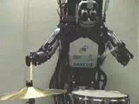
Fig. 8. Two-handed drumming using the Sarcos CB-i humanoid robot.
The control scheme was implemented in Matlab/Simulik and is presented in Fig. 9. The imitation system provides the desired task space trajectory for the robot’s arms. The waveform was defined in advance. Since the sound signal consists usually of several different tones, e.g. drums, guitar, singer, noise etc., it was necessary to pre-process the signal in order to get the periodic signal which represents the drumming. The input signal was modified into short pulses. This pre-processing only modifies the waveform and does not determine the frequency and the phase.
ydemo CDS
AF
AF
 wi
wi
ODS
xl,r
Music
Fig. 9. Proposed two-layered structure of the control system for synchronizing robotic drumming to the music.
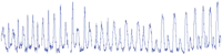
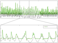
Fig. 10 shows the results of frequency adaptation to music. The waveforms for both hands were predefined. The frequency of the imitated motion quickly adapted to the drumming tones. The drumming sounds are presented with a real-time power spectrum. With this particular experiment we show the possibility of using our proposed system for synchronizing robot’s motion with an arbitrary periodic signal, e.g. music. Due to the complexity of the audio signal this experiment does require some modification of the measured (audio) signal, but is not pre-processed in the sense of determining the frequency. The drumming experiment shows that the proposed two-layered system is able to synchronize the motion of the robot to the drumming tones of the music.

6
![]() 4
4
2
0
0 10 20 30 40 50 60

1
![]() 0
0
−1
0 10 20 30 40 50 60
1 xl
 xr
xr
![]() 0
0
−1
25 30 35
t [s]
Fig. 10. Extracted frequency Ω of the drumming tones from the music in the top plot. Comparison between the power spectrum of the audio signal (drumming tones) y and robot trajectories for the left (xl ) and the right hand motions (xr ).
Table wiping
In this section we show how we can use the proposed two-layered system to modify already learned movement trajectories according to the measured force. ARMAR-IIIb humanoid robot, which is kinematically equal to the ARMAR-IIIa (Asfour et al., 2006) was used in the experiment.
From the kinematics point of view, the robot consists of seven subsystems: head, left arm, right arm, left hand, right hand, torso, and a mobile platform. The head has seven DOF and is equipped with two eyes, which have a common tilt and can pan independently. Each arm has 7 DOF and each hand additional 8DOF. The locomotion of the robot is realized using a wheel-based holonomic platform.
In order to obtain reliable motion data of a human wiping demonstration through observation by the robot, we exploited the color features of the sponge to track its motion. Using the stereo camera setup of the robot, the implemented blob tracking algorithm based on color segmentation and a particle filter framework provides a robust location estimation of the sponge in 3D. The resulting trajectories were captured with a frame rate of 30 Hz.
For learning of movements we first define the area of demonstration by measuring the lower-left and the upper-right position within a given time-frame, as is presented in Fig. 11. All tracked sponge-movement is then normalized and given as offset to the central position of this area.
For measuring the contact forces between the object in the hand and the surface of the plane a 6D-force/torque sensor is used, which is mounted at the wrist of the robot.
Adaptation of the learned trajectory using force feedback
Learning of a movement that brings the robot into contact with the environment must be based on force control, otherwise there can be damage to the robot or the object to which the robot applies its force. In the task of wiping a table, or any other object of arbitrary shape,
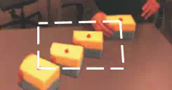 Fig. 11. Area for movement demonstration is determined by measuring the bottom-left most and the top-right most positions within a given time frame. These coordinates make a rectangular area (marked with dashed lines) where the robot tracks the demonstrated movements.
constant contact with the object is required. To teach the robot the necessary movement, we decoupled the learning of the movement from the learning of the shape of the object. We first apply the described two-layered movement imitation system to learn the desired trajectories by means of visual feedback. We then use force-feedback to adapt the motion to the shape of the object that the robot acts upon.
Periodic movements can be of any shape, yet wiping can be effective with simple one dimensional left-right movement, or circular movement. Once we are satisfied with the learned movement, we can reduce the frequency of the movement by modifying the Ω value. The low frequency of movement and consequentially low movement speed reduce the possibility of any damage to the robot. When performing playback we modify the learned movement with an active compliance algorithm. The algorithm is based on the velocity-resolved approach (Villani & J., 2008). The end-effector velocity is calculated by
vr = Sv vv + KF SF (Fm − F0 ).
(26) Here vr stands for the resolved velocities vector, Sv for the velocity selection matrix, vv for the
desired velocities vector, KF for the force gain matrix, SF for the force selection matrix, and
Fm for the measured force. F0 denotes the force offset which determines the behavior of the robot when not in contact with the environment. To get the desired positions we use
Y = Yr + SF vr dt.
(27) Here Yr is the desired initial position and Y = (yj ), j = 1, …, 6 is the actual
position/orientation. Using this approach we can modify the trajectory of the learned periodic
movement as described below.
Equations (26 – 27) become simpler for the specific case of wiping a flat surface. By using a null matrix for Sv , KF = diag(0, 0, kF , 0, 0, 0), SF = diag(0, 0, 1, 0, 0, 0), the desired end-effector height z in each discrete time step ∆t becomes
z˙ (t) = kF (Fz (t) − F0 ), (28)
z(t) = z0 + z˙ (t)∆t. (29)
Here z0 is the starting height, kF is the force gain (of units kg/s), Fz is the measured force in the z direction and F0 is the force with which we want the robot to press on the object. Such formulation of the movement ensures constant movement in the −z direction, or constant

upwards every time it hits something, for example the side of a sink. No contact should be made from above, as this will make the robot press up harder and harder.
The learning of the force profile is done by modifying the weighs wi for the selected degree of freedom yj in every time-step by incremental locally weighted regression (Atkeson et al.,
1997), see also Section 2.1.
The KF matrix controls the behavior of the movement. The correcting movement has to be fast enough to move away from the object if the robot hand encounters sufficient force, and at the same time not too fast so that it does not produce instabilities due to the discrete-time sampling when in contact with an object. A dead-zone of response has to be included, for example |F| < 1 N, to take into account the noise. We empirically set kF = 20, and limited the force feedback to allow maximum linear velocity of 120 mm/s.
Feedback from a force-torque sensor is often noisy due to the sensor itself and mainly due to vibrations of the robot. A noisy signal is not the best solution for the learning algorithm because we also need time-discrete first and second derivatives. The described active compliance algorithm uses the position of the end-effector as input, which is the integrated desired velocity and therefore has no difficulties with the noisy measured signal.
Having adapted the trajectory to the new surface enables very fast movement with a constant force profile at the contact of the robot/sponge and the object, without any time-sampling and instability problems that may arise when using compliance control only. Furthermore, we can still use the compliant control once we have learned the shape of the object. Active compliance, combined with a passive compliance of a sponge, and the modulation and perturbation properties of DMPs, such as slow-down feedback, allow fast and safe execution of periodic movement while maintaining a sliding contact with the environment.
The learning scenario
Our kitchen scenario includes the ARMAR-IIIb humanoid robot wiping a kitchen table. First the robot attempts to learn wiping movement from human demonstration. During the demonstration of the desired wiping movement the robot tracks the movement of the sponge in the demonstrator ’s hand with his eyes. The robot only reads the coordinates of the movement in a horizontal plane, and learns the frequency and waveform of the movement. The waveform can be arbitrary, but for wiping it can be simple circular or one-dimensional left-right movement. The learned movement is encoded in the task space of the robot, and an inverse kinematics algorithm controls the movement of separate joints of the 7-DOF arm. The robot starts mimicking the movement already during the demonstration, so the demonstrator can stop learning once he/she is satisfied with the learned movement. Once the basic learning of periodic movement is stopped, we use force-feedback to modify the learned trajectory. The term F − F0 in (28) provides velocity in the direction of −z axis, and the hand holding the sponge moves towards the kitchen table or any other surface under the arm. As the hand makes contact with the surface of an object, the vertical velocity adapts. The force profile is learned in a few periods of the movement. The operator can afterwards stop force profile learning and execute the adjusted trajectory at an arbitrary frequency.
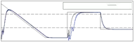
Fig. 12 on the left shows the results of learning the force-profile for a flat surface. As the robot grasps the sponge, its orientation and location are unknown to the robot, and the tool center point (TCP) changes. Should the robot simply perform a planar trajectory it would not ensure constant contact with the table. As we can see from the results, the hand initially
−250
![]() −300
−300
![]() −350
−350
 −250
−250
![]() −300
−300
−350
−400

0 5 10 15 20 25 30 35 40
−400

0 20 40 60 80 100
8 8
 6 6
6 6
![]()
![]() 4 4
4 4
2 2
![]() 0 0
0 0
−2
0 5 10 15 20 25 30 35 40
t [s]
−2
0 20 40 60 80 100
 t [s]
t [s]
Fig. 12. Results of learning the force profile on a flat surface on the left and on a bowl-shaped surface on the right. For the flat surface we can see that the height of the movement changes for approx. 5 cm during one period to maintain contact with the surface. The values were attained trough robot kinematics. For the bowl shaped surface we can see that the trajectory assumes a bowl-shape with an additional change of direction, which is the result of the compliance of the wiping sponge and the zero-velocity dead-zone. A dashed vertical line marks the end of learning of the force profile. Increase in frequency can be observed in the end of the plot. The increase was added manually.

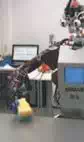


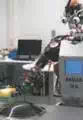


Fig. 13. A sequence of still photos showing the adaptation of wiping movement via force-feedback to a flat surface, as of a kitchen table, in the top row, and adaptation to a bowl-shaped surface in the bottom row.
moves down until it makes contact with the surface. The force profile later changes the desired height by approx. 5 cm within one period. After the learning (stopped manually, marked with a vertical dashed line) the robot maintains such a profile. A manual increase in frequency was introduced to demonstrate the ability to perform the task at an arbitrary frequency. The
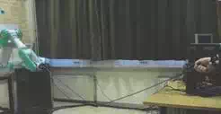
Fig. 14. Experimental setup for cooperative human-robot rope turning.
bottom plot shows the measured length of the force vector |F|. As we can see the force vector keeps the same force profile, even though the frequency is increased. No increase in the force profile proves that the robot has learned the required trajectory. Fig. 13 shows a sequence of photos showing the adaptation to the flat and bowl-shaped surfaces.
Fig. 12 on the right shows the results for a bowl-shaped object. As we can see from the results the height of the movement changes for more than 6 cm within a period. The learned shape (after the vertical dashed lined) maintains the shape of a bowl, but has an added local minimum. This is the result of the dead-zone within the active compliance, which comes into effect when going up one side, and down the other side of the bowl. No significant change in the force profile can be observed in the bottom plot after a manual increase in frequency. Some drift, as the consequence of an error of the sensor and of wrist control on the robot, can be observed.
Synchronization with external signals
Once the movement is learned we can change its frequency. The new frequency can be determined from an external signal using the canonical dynamical system. This allows easy synchronization to external measured signals, such as drumming, already presented in Section 3.3. In this section we show how we applied the system to a rope turning task, which is task that requires continuous cooperation of a human and a robot. We also show how we can synchronize to an EMG signal, which is inherently very noisy.
Robotic rope turning
We performed the rope-turning experiment on a Mitsubishi PA-10 robot with a JR-3 force/torque sensor attached to the top of the robot to measure the torques and forces in the string. Additionally, an optical system (Optotrak Certus) was used for validation, i.e. for measuring the motion of a human hand. The two-layered control system was implemented in Matlab/Simulink. The imitation system provides a pre-defined desired circular trajectory for the robot. The motion of a robot is constrained to up-down and left-right motion using inverse kinematics. Figure 14 shows the experimental setup.
Determining the frequency is done using the canonical dynamical system. Fig. 15 left shows the results of frequency extraction (top plot) from the measured torque signal (second plot). The frequency of the imitated motion quickly adapts to the measured periodic signal. When the rotation of the rope is stable, the human stops swinging the rope and maintains the hand in a fixed position. The movement of the human hand is shown in the third plot. In the last plot we show the movement of the robot. By comparing the last two plots in Fig. 15 left, we can see that after 3 s the energy transition to the rope is done only by the motion of the robot.
The frequency of the task depends on the parameters of the rope, i.e. weight, length, flexibility etc., and the energy which is transmitted in to the rope. The rotating frequency of the rope can be influenced by the amplitude of the motion, i.e. how much energy is transmitted to the rope. The amplitude can be easily modified with the amplitude parameter r.
Fig. 15 right shows the behavior of the system, when the distance between the human hand and the top end of the robot (second plot) is changing, while the length of the rope remains the same, consequently the rotation frequency changes. The frequency adaptation is shown in the top plot. As we can see, the robot was able to rotate the rope and maintain synchronized even if disturbances like changing the distance between the human hand and the robot occur. This shows that the system is adaptable and robust.
EMG based human-robot synchronization
In this section we show the results of synchronizing robot movement to an EMG signal measured from the human biceps muscle. More details can be found at (Petricˇ et al., 2011). The purpose of this experiment is to show frequency extraction from a signal with a low signal-to-noise ratio. This type of applications can be used for control of periodic movements of limb prosthesis (Castellini & Smagt, 2009) or exoskeletons.
In our experimental setup we attached an array of 3 electrodes (Motion Control Inc.) over the biceps muscle of a subject and asked the subject to flex his arm when he hears a beep. The frequency of beeping was 1 Hz from the start of the experiment, then changed to 0.5 Hz after 30 s, and then back to 1 Hz after additional 30 s. Fig. 16 left shows the results of frequency
![]() 18
18
![]() 16
16
14
12
10
8
![]()
![]() 1
1
0
−1
0.2
![]() 0
0 ![]()
−0.2
![]() 18
18
![]() 16
16
14
12
10
8
![]() 1.6
1.6
1.4
1.2
1
![]()
![]() 0.8
0.8
0.2
0 ![]()
−0.2
![]() 0.1
0.1
0
−0.1
![]() 0 1 2 3 4 5 6 7
0 1 2 3 4 5 6 7
t [s]
0.1
0
![]() −0.1
−0.1

0 10 20 30 40
t [s]
Fig. 15. Left: the initial frequency adaptation process (top plot) of the cooperative
human-robot rope turning. The second plot shows the measured torque signal. The third plot shows the movement of a human hand, and the bottom plot shows the movement of a robot. Right: the behavior of our proposed system when human changes the distance between human hand and top end of the robot. Frequency adaptation is shown in the top plot, and the second plot shows the measured torque signal. The third plot shows the movement of a human hand, and the bottom plot shows the movement of a robot.
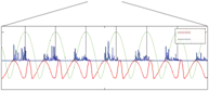
extraction (third plot) from the envelope (second plot) of the measured EMG signal (top plot). The bottom plots show the power spectrums of the input signal from 0 s to 30 s, from 30 s to 60 s and from 60 s to 90 s, respectively. The power spectrums were determined off-line.
 AF
AF
ydemo CDS
AF
wi
ODS x
EMG
l r
HOAP-3
Fig. 16. Proposed two-layered structure of the control system for synchronizing the robotic motion to the EMG signal.


![]() 0 30 60 90
0 30 60 90
0 30 60 90


![]() 5
5 ![]()
![]() 0
0

 0 30 60 90
 t [s]
t [s]
 8
8
![]() 6
6
4
2
0
0 30 60 90
0.6
![]() 0.4
0.4
0.2
0
−0.2
 0 30 60 90
x y
0 5 10 15
Ω [rad]
0 5 10 15
Ω [rad]
0 5 10 15
Ω [rad]
![]() 0.4
0.4
0.2
0
−
30 35 40 45
t [s]
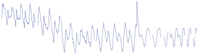
Fig. 17. Left:Raw EMG signal in the top plot and envelope of the EMG signal, which is the input into the proposed system, in the second plot. The third plot shows the extracted frequency Ω. The bottom plots show the power spectrum of the signal at different times (determined off-line). Right: Extracted frequency in the top plot. Comparison between the envelope of the rectified EMG signal (y), which is used as the input into the frequency-extraction system, and the generated output trajectory for the robot arm (x) is shown in the middle and bottom plots.
Fig. 17 right show the comparison between the envelope of the measured and rectified EMG signal (y), and the generated movement signal (x). As we can see the proposed system matches the desired movement of the robot with the measured movement.
Conclusion
We have shown the properties and the possible use of the proposed two-layered movement imitation system. The system can be used for both waveform learning and frequency extraction. Each of these has preferable properties for learning and controlling of robots by imitation. On-line waveform learning can be used for effective and natural learning of robotic movement, with the demonstrator in the loop. During learning the demonstrator can observe the learned behavior of the robot and if necessary adapt his movement to achieve better robot performance. The table wiping task is an example of such on-line learning, where not only is the operator in the loop for the initial trajectory, but online learning adapts the trajectory based on the measured force signal.
Online frequency extraction, essential for waveform learning, can additionally be used for synchronization to external signals. Examples of such tasks are drumming, cooperative rope turning and synchronization to a measured EMG signal. Specially the synchronization to an EMG signal shows at great robustness of the system. Furthermore, the process of synchronizing the movement of the robot and the actuated device can be applied in a similar manner to different tasks and can be used as a common generic algorithm for controlling periodic tasks. It is also easy to implement, with hardly any parameter tuning at all.
The overall structure of the system, based on nonlinear oscillators and dynamic movement primitives is, besides computationally extremely light, also inherently robust. The properties of dynamic movement primitives, which allow on-line modulation, and return smoothly to the desired trajectory after perturbation, allow learning of whole families of movement with one demonstrated trajectory. An example of such is learning of circular movement, which can be increased in amplitude, or we can change the center of the circular movement. Additional modifications, such as slow-down feedback and virtual repulsive forces even expand these properties into a coherent and complete block for control of periodic robotic movements.


Comments are closed