
This paper describes the methodology for system description and application so that the system can be managed using real time system adaptation. The term system here can represent any structure regardless its size or complexity (industrial robots, mobile robot navigation, stock market, systems of production, control systems, etc.). The methodology describes the whole development process from system requirements to software tool that will be able to execute a specific system adaptation.
In this work, we propose approaches relying on machine learning methods (Bishop, 2006), which would enable to characterize key patterns and detect them in real time and in their altered form as well. Then, based on the pattern recognized, it is possible to apply a suitable intervention to system inputs so that the system responds in the desired way. Our aim is to develop and apply a hybrid approach based on machine learning methods, particularly based on soft-computing methods to identify patterns successfully and for the subsequent adaptation of the system. The main goal of the paper is to recognize important pattern and adapt the system’s behaviour based on the pattern desired way.
The paper is arranged as follows: Section 1 introduces the critical topic of the article. Section 2 details the feature extraction process in order to optimize the patterns used as inputs into experiments. The pattern recognition algorithms using machine learning methods are discussed in section 3. Section 4 describes the used data-sets and covers the experimental results and a conclusion is given in section 5. We focus on reliability of recognition made by the described algorithms with optimized patterns based on the reduction of the calculation costs. All results are compared mutually.
The methodology for system description
Gershenson (Gershenson, 2007) proposed a methodology called The General Methodology for system description necessary to manage a system. It presents a conceptual framework for describing systems as self-organizing and consists of five steps: representation, modelling, simulation, application and evaluation. Our goal is to use and adapt this methodology for our specific needs. Basically we would like to describe a methodology that the designer should be able to use to describe his system, find key patterns in its behaviour based on the observation and prepare suitable response to these patterns that emerge from time to time and adapt to any deviation in the system’s behaviour.
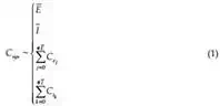
As we are using Gershenson’s methodology we are not going to describe it in detail because detailed info can be found in his book (Gershenson, 2007). Let’s mention crucial parts of his methodology that is important to our work. The methodology is useful for designing and controlling complex systems. Basically a complex system consists of two or more interconnected components and these components react together and it is very complicated to separate them. So the system’s behaviour is impossible to deduce from the behaviour of its individual components. This deduction becomes more complicated how more![]() components
components
#E and more interactions
#I the system has (Csys corresponds with system
complexity; Ce corresponds with element complexity; Ci corresponds with interaction complexity).
Imagine a manufacturing factory. We can describe the manufacturing factory as a complex system. Now it is important to realize that we can have several levels of abstraction starting from the manufacturing line to the whole factory complex. The manufacturing line can consist of many components. There can be robots, which perform the main job. Conveyor belts, roller beds, jigs, hangers and other equipment responsible for the product or material transport and other equipments. All the interactions are some way related to the material or product. Although it is our best interest to run all the processes smoothly there will be always some incidents we cannot predict exactly. The supply of the material can be interrupted or delayed, any equipment can have a multifunction and it is hard to predict when and how long will it takes. Because there are interactions among many of these components we can call manufacturing factory a complex system.
If we want to characterize a system we should create its model. Gershenson (Gershenson, 2002) proposes two types of models, absolute and relative. The absolute model (abs-model) refers to what the thing actually is, independently of the observer. The relative model (rel- model) refers to the properties of the thing as distinguished by an observer within a context. We can say that the rel-model is a model, while the abs-model is modelled. Since we are all limited observers, it becomes clear that we can speak about reality only with rel- beings/models (Gershenson, 2007).
So how we can model a complex system? Any complex system can be modelled using multi- agent system (MAS) where each system’s component is represented by an agent and any interactions among system’s components are represented as interactions among agents. If we take into consideration The General Methodology thus any system can be modelled as group of agents trying to satisfy their goals. There is a question. Can we describe a systems modelling as a group of agents as self-organizing? We think that we can say Yes. As the agents in the MAS try to satisfy their goals, same as components in self-organizing systems interact with each other to achieve desired state or behaviour. If we determine the state as a self-organizing state, we can call that system self-organizing and define our complex self-organizing system. In our example with manufacturing line our self-organizing state will be a state where the production runs smoothly without any production delays. But how can we achieve that?
Still using Gerhenson’s General Methodology we can label fulfilling agent’s goal as its satisfaction σ ∈ [0,1]. Then the system’s satisfaction σsys (2) can be represented as function f : R → [0 , 1] and it is a satisfaction of its individual components.
σsys = f (σ1, σ2,…, σn, w0,w1, w2, …, wn) (2)
w0 represents bias and other weights wi represents an importance given to each σi. Components, which decrease σsys and increase their σi shouldn’t be considered as a part of the system. Of course it is hard to say if for higher system’s satisfaction it is sufficient to increase satisfaction of each individual component because some components can use others fulfilling their goals. For maximization of σsys we should minimize the friction among components and increase their synergy. A mediator arbitrates among elements of a system, to minimize conflict, interferences and frictions; and to maximize cooperation and synergy. So we have two types of agents in the MAS. Regular agents fulfil their goals and mediator agents streamline their behaviour. Using that simple agent’s division we can build quite adaptive system.
Patterns as a system’s behaviour description
Every system has its unique characteristics that can be described as patterns. Using patterns we would like to characterize particular system and its key characteristics. Generally a system can sense a lot of data using its sensors. If we put the sensor’s data into some form, a set or a graph then a lot of patterns can be recognized and further processed. When every system’s component has some sensor then the system can produce some patterns in its behaviour. Some sensor reads data about its environment so we can find some patterns of the environment, where the system is located. If we combine several sensors data, we would be able to recognise some patterns in the whole system’s behaviour. It is important to realize that everything, which we observe is relative from our point of view. When we search for the pattern, we want to choose such pattern, which represents the system reliably and define its important properties. Every pattern, which we find, is always misrepresented with our point of view.
We can imagine a pattern as some object with same or similar properties. There are many ways how to recognize and sort them. When we perform pattern recognition, we assign a pre-defined output value to an input value. For some purpose, we can use a particular pattern recognition algorithm, which is introduced in (Ciskowski & Zaton, 2010). In this case we try to assign each input value to the one of the output sets of values. Some input value can be any data regardless its origin as a text, audio, image or any other data. When patterns repeat in the same or altered forms then can be classified into predefined classes of patterns. Since we are working on computers, the input data and all patterns can be represented in a binary form without the loss of generality. Such approach can work nearly with any system, which we would like to describe. But that is a very wide frame content.
Although theory of regulation and control (Armstrong & Porter, 2006) is mainly focused on methods of automatic control, it also includes methods for adaptive and fuzzy controls. In general, through the control or regulation we guide the system’s behaviour in the desired direction. For our purposes, it suffices to regulate the system behaviour based on the predefined target and compensate any deviation in desired direction. So we search for key patterns in system’s behaviour a try to adapt to any changes. However, in order to react quickly and appropriately, it is good to have at least an expectation of what may happen and which reaction would be appropriate, i.e. what to anticipate. Expectations are subjective probabilities that we learn from experience: the more often pattern B appears after pattern A, or the more successful action B is in solving problem A, the stronger the association A → B becomes. The next time we encounter A (or a pattern similar to A), we will be prepared, and more likely to react adequately. The simple ordering of options according to the probability that they would be relevant immensely decreases the complexity of decision- making (Heylighen, 1994).
Agents are appropriate for defining, creating, maintaining, and operating the software of distributed systems in a flexible manner, independent of service location and technology. Systems of agents are complex in part because both the structural form and the behaviour patterns of the system change over time, with changing circumstances. By structural form, we mean the set of active agents and inter-agent relationships at a particular time. This form changes over time as a result of inter-agent negotiations that determine how to deal with new circumstances or events. We call such changing structural form morphing, by analogy with morphing in computer animation. By behaviour patterns, we mean the collaborative behaviour of a set of active agents in achieving some overall purpose. In this sense, behaviour patterns are properties of the whole system, above the level of the internal agent detail or of pair wise, inter-agent interactions. Descriptions of whole system behaviour patterns need to be above this level of detail to avoid becoming lost in the detail, because agents are, in general, large grained system components with lots of internal detail, and because agents may engage in detailed sequences of interactions that easily obscure the big picture. In agent systems, behaviour patterns and morphing are inseparable, because they both occur on the same time scale, as part of normal operation. Use case maps (UCMs) (Burth & Hubbard, 1997) are descriptions of large grained behaviour patterns in systems of collaborating large grained components.
System adaptation vs. prediction
Let’s say we have built pattern recognition system and it is working properly to meet our requirements. We are able to recognize certain patterns reliably. What can we do next? Basically, we can predict systems behaviour or we can adapt to any change that emerge.
It is possible to try to predict what will happen, but more or less it is a lottery. We will never be able to predict such systems’ behaviour completely. This doesn’t mean it is not possible to build a system based on prediction (Gershenson, 2007). But there is another approach that tries to adapt to any change by reflecting current situation. To adapt on any change (expected or unexpected) it should be sufficient to compensate any deviation from desired course. In case that response to a deviation comes quickly enough that way of regulation can be very effective. It does not matter how complicated system is (how many factors and interactions has) in case we have efficient means of control (Armstrong & Porter, 2006). To respond quickly and flexible it is desirable to have some expectation what can happen and what kind of response will be appropriate. We can learn such expectation through experiences.
Feature extraction process in order to optimize the patterns
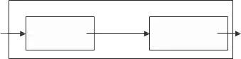
Identification problems involving time-series data (or waveforms) constitute a subset of pattern recognition applications that is of particular interest because of the large number of domains that involve such data. The recognition of structural shapes plays a central role in distinguishing particular system behaviour. Sometimes just one structural form (a bump, an abrupt peak or a sinusoidal component), is enough to identify a specific phenomenon. There is not a general rule to describe the structure – or structure combinations – of various phenomena, so specific knowledge about their characteristics has to be taken into account. In other words, signal structural shape may be not enough for a complete description of system properties. Therefore, domain knowledge has to be added to the structural information. However, the goal of our approach is not knowledge extraction but to provide users with an easy tool to perform a first data screening. In this sense, the interest is focused on searching for specific patterns within waveforms (Dormido-Canto et al., 2006). The algorithms used in pattern recognition systems are commonly divided into two tasks, as shown in Fig. 1. The description task transforms data collected from the environment into features (primitives).
Pattern Recognition Algorithms
data
features
 Description Classification
Identification
Fig. 1. Tasks in the pattern recognition systems
The classification task arrives at an identification of patterns based on the features provided by the description task. There is no general solution for extracting structural features from data. The selection of primitives by which the patterns of interest are going to be described depends upon the type of data and the associated application. The features are generally designed making use of the experience and intuition of the designer.
The input data can be presented to the system in various forms. In principle we can distinguish two basic possibilities:
• The numeric representation of monitored parameters
• Image data – using the methods of machine vision
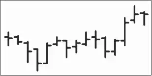 Figures 2 and 3 show an image and a numerical expression of one particular section of OHLC data. The image expression contains only information from the third to the sixth column of the table (Fig.3). In spite of the fact, the pattern size (number of pixels) equals to 7440. In contrast to it, a table expression with 15 rows and 7 columns of 16-bit numbers takes only.
Fig. 2. Visual representations of pattern
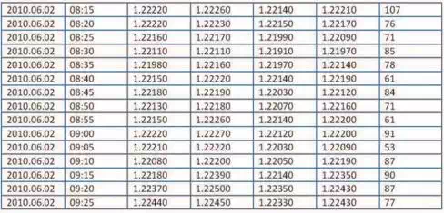
Fig. 3. Tabular expression of pattern
The image data better correspond to an intuitive human idea of patterns recognitions, which is their main advantage. We also have to remember that even table data must be transferred into binary (image) form before their processing.
Image data are always two-dimensional. Generally, tabular patterns can have more dimensions. Graphical representation of OHLC data (Lai, 2005) in Fig.2 is a good example of the expression of multidimensional data projection to two-dimensional space. Fig.2 shows a visual representation of 4-dimensional vector in time, which corresponds to 5 – dimensions. In this article, we consider experiments only over two-dimensional data (time series). Extending the principles of multidimensional vectors (random processes) will be the subject of our future projects.
The intuitive concept of “pattern” corresponds to the two-dimensional shapes. This way allows showing a progress of a scalar variable. In the case that a system has more than one parameter, the graphic representation is not trivial anymore.
Pattern recognition algorithms
Classification is one of the most frequently encountered decision making tasks of human activity. A classification problem occurs when an object needs to be assigned into a predefined group or class based on a number of observed attributes related to that object. Pattern recognition is concerned with making decisions from complex patterns of information. The goal has always been to tackle those tasks presently undertaken by humans, for instance to recognize faces, buy or sell stocks or to decide on the next move in a chess game. Rather simpler tasks have been considered by us. We have defined a set of classes, which we plan to assign patterns to, and the task is to classify a future pattern as one of these classes. Such tasks are called classification or supervised pattern recognition. Clearly someone had to determine the classes in the first phase. Seeking the groupings of patterns is called cluster analysis or unsupervised pattern recognition. Patterns are made up of features, which are measurements used as inputs to the classification system. In case that patterns are images, the major part of the design of a pattern recognition system is to select suitable features; choosing the right features can be even more important than what is done with them subsequently.
Artificial neural networks
Neural networks that allow so-called supervised learning process (i.e. approach, in which the neural network is familiar with prototype of patterns) use to be regarded as the best choice for pattern recognition tasks. After adaptation, it is expected that the network is able to recognise learned (known) or similar patterns in input vectors. Generally, it is true – the more training patterns (prototypes), the better network ability to solve the problem. On the other hand, too many training patterns could lead to exceeding a memory capacity of the network. We used typical representative of neural networks, namely:
• Hebb network
• Backpropagation network
Our aim was to test two networks with extreme qualities. In other words, we chose such neural networks, which promised the greatest possible differences among achieved results.
Hebb network
Hebb network is the simplest and also the “cheapest” neural network, which adaptation runs in one cycle. Both adaptive and inactive modes work with integer numbers. These properties allow very easy training set modification namely in applications that work with very large input vectors (e.g. image data).
Hebbian learning in its simplest form (Fausett, 1994) is given by the weights update rule (3)
Δwij = η ai aj (3)
where wij is the change in the strength of the connection from unit j to unit i, ai and aj are the activations of units i and j respectively, and η is a learning rate. When training a network to classify patterns with this rule, it is necessary to have some method of forcing a unit to respond strongly to a particular pattern. Consider a set of data divided into classes C1, C2,…,Cm.
Each data point x is represented by the vector of inputs (x1, x2, …, xn). A possible network for learning is given in Figure 4. All units are linear. During training the class inputs c1, c2, …,cm for a point x are set as follows (4):
ci = 1
ci = 0
x ∈ Ci
x ∉ Ci
(4)
Each of the class inputs is connected to just one corresponding output unit, i.e. ci connects to oi only for i = 1, 2, …,m. There is full interconnection from the data inputs x1, x2, …, xn to each of these outputs.
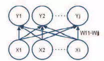
Fig. 4. Hebb network. Weights of connections w11-wij are modified in accordance with the
Hebbian learning rule
Backpropagation network
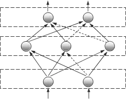
Back propagation network is one of the most complex neural networks for supervised learning. Its ability to learning and recognition are much higher than Hebb network, but its disadvantage is relatively lengthy processes of adaptation, which may in some cases (complex input vectors) significantly prolong the network adaptation to new training sets. Backpropagaton network is a multilayer feedforward neural network. See Fig. 5, usually a fully connected variant is used, so that each neuron from the n-th layer is connected to all neurons in the (n+1)-th layer, but it is not necessary and in general some connections may be missing – see dashed lines, however, there are no connections between neurons of the same layer. A subset of input units has no input connections from other units; their states are fixed by the problem. Another subset of units is designated as output units; their states are considered the result of the computation. Units that are neither input nor output are known as hidden units.
output
 hidden
input
Fig. 5. A general three-layer neural network
Backpropagation algorithm belongs to a group called “gradient descent methods”. An intuitive definition is that such an algorithm searches for the global minimum of the weight landscape by descending downhill in the most precipitous direction. The initial position is set at random selecting the weights of the network from some range (typically from -1 to 1 or from 0 to 1). Considering the different points, it is clear, that backpropagation using a fully connected neural network is not a deterministic algorithm. The basic backpropagation algorithm can be summed up in the following equation (the delta rule) for the change to the weight wji from node i to node j (5):
weight change
learning rate
local gradient
input signal to node j
(5)
Δwji = η × δj × yi
where the local gradient δj is defined as follows: (Seung, 2002):
1. If node j is an output node, then δj is the product of φ'(vj) and the error signal ej, where φ(_) is the logistic function and vj is the total input to node j (i.e. Σi wjiyi), and ej is the error signal for node j (i.e. the difference between the desired output and the actual output);
2. If node j is a hidden node, then δj is the product of φ'(vj) and the weighted sum of the δ’s computed for the nodes in the next hidden or output layer that are connected to node j.
[The actual formula is δj = φ'(vj) &Sigmak δkwkj where k ranges over those nodes for which wkj is non-zero (i.e. nodes k that actually have connections from node j. The δk values have already been computed as they are in the output layer (or a layer closer to the output layer than node j).]
Analytic programming
Basic principles of the analytic programming (AP) were developed in 2001 (Zelinka, 2002). Until that time only genetic programming (GP) and grammatical evolution (GE) had existed. GP uses genetic algorithms while AP can be used with any evolutionary algorithm, independently on individual representation. To avoid any confusion, based on use of names according to the used algorithm, the name – Analytic Programming was chosen, since AP represents synthesis of analytical solution by means of evolutionary algorithms.
The core of AP is based on a special set of mathematical objects and operations. The set of mathematical objects is set of functions, operators and so-called terminals (as well as in GP), which are usually constants or independent variables. This set of variables is usually mixed together and consists of functions with different number of arguments. Because of a variability of the content of this set, it is called here “general functional set” – GFS. The structure of GFS is created by subsets of functions according to the number of their arguments. For example GFSall is a set of all functions, operators and terminals, GFS3arg is a subset containing functions with only three arguments, GFS0arg represents only terminals, etc. The subset structure presence in GFS is vitally important for AP. It is used to avoid synthesis of pathological programs, i.e. programs containing functions without arguments, etc. The content of GFS is dependent only on the user. Various functions and terminals can be mixed together (Zelinka, 2002; Oplatková, 2009).
The second part of the AP core is a sequence of mathematical operations, which are used for the program synthesis. These operations are used to transform an individual of a population into a suitable program. Mathematically stated, it is a mapping from an individual domain into a program domain. This mapping consists of two main parts. The first part is called discrete set handling (DSH), see Fig. 6 (Zelinka, 2002) and the second one stands for security procedures which do not allow synthesizing pathological programs. The method of DSH, when used, allows handling arbitrary objects including nonnumeric objects like linguistic terms {hot, cold, dark…}, logic terms (True, False) or other user defined functions. In the AP DSH is used to map an individual into GFS and together with security procedures creates the above mentioned mapping which transforms arbitrary individual into a program.
AP needs some evolutionary algorithm (Zelinka, 2004) that consists of population of individuals for its run. Individuals in the population consist of integer parameters, i.e. an individual is an integer index pointing into GFS. The creation of the program can be schematically observed in Fig. 7. The individual contains numbers which are indices into GFS. The detailed description is represented in (Zelinka, 2002; Oplatková, 2009).
AP exists in 3 versions – basic without constant estimation, APnf – estimation by means of nonlinear fitting package in Mathematica environment and APmeta – constant estimation by means of another evolutionary algorithms; meta means metaevolution.
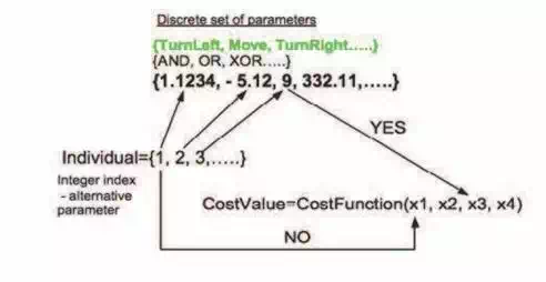
Fig. 6. Discrete set handling
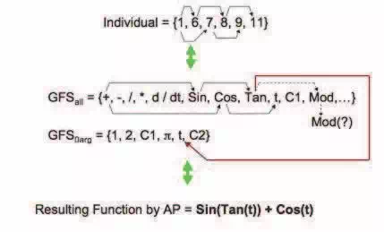
Fig. 7. Main principles of AP
Experimental results
Used datasets
This approach allows a search of structural shapes (patterns) inside time-series. Patterns are composed of simpler sub-patterns. The most elementary ones are known as primitives. Feature extraction is carried out by dividing the initial waveform into segments, which are encoded. Search for patterns is accomplished process, which is performed manually by the user. In order to test the efficiency of pattern recognition, we applied a database downloaded from (Google finance, 2010). We used time series, which shows development of the market value of U.S. company Google and represents the minute time series from 29 October 2010, see Fig. 8.
Used algorithms need for their adaptation training sets. In all experimental works, the training set consists of 100 samples (e.g. training pars of input and corresponding output vectors) and it is made from the time series and contains three peaks, which are indicated by vertical lines and they are shown in Figure 8. Samples obtained in this way are always adjusted for the needs of the specific algorithm. Data, which were tested in our experimental works, contains only one peak, which is indicated by vertical lines and it is shown in Fig. 9.
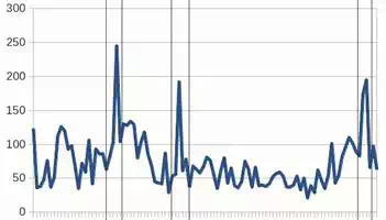
Fig. 8. The training set with three marked peaks
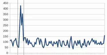
Fig. 9. The test set with one marked peak, which is searched
Pattern recognition via artificial neural networks
The aim of this experiment was to adapt neural network so that it could find one kind of pattern (peak) in the test data. We have used two sets of values, which are graphically depicted in Figure 10 (training patterns) and Figure 11 (test patterns) in our experiments. Training set always contained all define peaks, which were completed by four randomly selected parts out of peaks. These randomly selected parts were used to network can learn to recognize what is or what is not a search pattern (peak). All patterns were normalized to the square of a bitmap of the edge of size a = 10. The effort is always to choose the size of training set as small as possible, because especially backpropagation networks increases their computational complexity with the size of a training set.

Fig. 10. Graphic representation of learning patterns (S vectors) that have been made by selection from training data set. The first three patterns represent peaks. Next four patterns are representatives of non-peak “not-interested” segments of values
| No. | S | T |
| 0. | ——–+-|——-++-|——-+++|——++++|——++++|—–+++++|—–+++++|–++++++++|++++++++++|++++++++++ | -+ |
| 1. | ———-|———-|——–+-|——-++-|——-+++|——++++|——++++|—–+++++|—–+++++|–++++++++ | -+ |
| 2. | ———-|———-|——-++-|—–++++-|—-++++++|—-++++++|—+++++++|++++++++++|++++++++++|++++++++++ | -+ |
| 3. | ———-|———-|———-|———-|———-|———-|———-|———-|——-+++|++++++++++ | +- |
| 4. | ———-|———-|———-|———-|———-|———-|———-|———-|———-|+++++++++- | +- |
| 5. | ———-|———-|———-|———-|———-|———-|——–++|——-+++|++—-++++|++++++++++ | +- |
| 6. | ———-|———-|———-|———-|———-|———-|——–+-|——++++|–++++++++|++++++++++ | +- |
Table 1. Vectors T and S from the learning pattern set. Values of ‘-1’ are written using the character ‘-’ and values of ‘+1’ are written using the character ‘+’ because of better clarity

Fig. 11. Graphic representation of test patterns (S vectors) that have been made by selection from the test data set. The first pattern represents the peak. Next four patterns are representatives of non-peak “not-interested” segments of values
| No. | S | T |
| 0. | —+——|–+++—–|–+++—+-|-++++++++-|-+++++++++|++++++++++|++++++++++|++++++++++|++++++++++|++++++++++ | -+ |
| 1. | ———-|———-|———-|———-|———-|———-|———-|—–+—-|—+++++–|-++++++++- | +- |
| 2. | ———-|———-|———-|———-|———-|———-|———-|———-|—–++—|–++++++++ | +- |
| 3. | ———-|———-|———-|———-|———-|———-|———-|———-|—++++—|-+++++++++ | +- |
| 4. | ———-|———-|———-|———-|———-|———-|———-|———-|+++++++++-|++++++++++ | +- |
Table 2. Vectors T and S from the test pattern set. Values of ‘-1’ are written using the character ‘-’ and values of ‘+1’ are written using the character ‘+’ because of better clarity
Two types of classifiers: Backpropagation and classifier based on Hebb learning were used in our experimental part. Both used networks classified input patterns into two classes. Backpropagation network was adapted according the training set (Fig.10, Tab. 1) in 7 cycles. After its adaptation, the network was able to also correctly classify all five patterns from the test set (Fig. 11, Tab. 2), e.g. the network was able to correctly identify the peak and “uninteresting” data segments too. Other experiments gave similar results too.
Backpropagation network configuration:
| Number of input neurons: | 100 |
| Number of output neurons: | 2 |
| Number of hidden layers: | 1 |
| Number of hidden neurons: | 3 |
| α – learning parameter: | 0.4 |
| Weight initialization algorithm: | Nguyen-Widrow |
| Weight initialization range: | (-0.5; +0.5) |
| Type of I/O values: | bipolar |
Hebb network in its basic configuration was not able to adapt given training set (Fig.10,
Tab. 1), therefore we used modified version of the network removing useless components from input vectors (Kocian & Volná & Janošek & Kotyrba, 2011). Then, the modified Hebb network was able to adapt all training patters (Fig. 12) and in addition to that the network correctly classified all the patterns from the test set (Fig. 11, Tab. 2), e.g. the network was able to correctly identify the peak and “uninteresting” data segments too. Other experiments gave similar results too.
Hebbian-learning-based-classifier configuration:
| Number of input neurons: | 100 |
| Number of output neurons: | 2 |
| Type of I/O values: | bipolar |

Fig. 12. Learning patterns from Fig. 10 with uncovered redundant components (gray colour). The redundant components prevented the Hebbian-learning-based-classifier in its default variant to learn patterns properly. So the modified variant had to be used
Pattern recognition via analytic programming
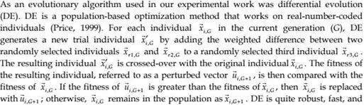
effective, with global optimization ability. It does not require the objective function to be differentiable, and it works well even with noisy and time-dependent objective functions. The technique for the solving of this problem by means of analytic programming was inspired in neural networks. The method in this case study used input values and future output values – similarly as training set for the neural network and the whole structure which transfer input to output was synthesized by analytic programming. The final solution of the analytic programming is based on evolutionary process which selects only the required components from the basic sets of operators (Fig. 6 and Fig 7). Fig. 13 shows analytic programming experimental result for exact modelling during training phase.
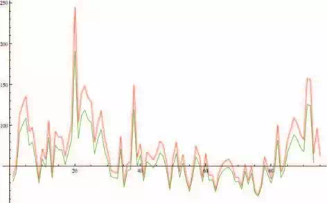
Fig. 13. Analytic programming experimental result for exact modelling during training phase. Red colour represents original data from training set (Fig. 8), while green colour represents modelling data using formula (6)
The resulting formula, which calculates the output value xn was developed using AP (6):
xn = 85.999 ⋅ e
(17.1502 − xn−3 )0.010009⋅xn−2
(6)
Analytic programming experimental results are shown in Fig. 14. Equation (6) also represents the behaviour of training set so that the given pattern was also successfully identified in the test set (Fig. 9). Other experiments gave similar results too.
The operators used in GFS were (see Fig. 7): +, -, /, *, Sin, Cos, K, xn-1 to xn-4, exp, power. As the main algorithm for AP and also for constants estimation in meta-evolutionary process differential evolution was used. The final solution of the analytic programming is based on evolutionary process which selects only the required components from the basic sets of operators. In this case, not all components have to be selected as can be seen in one of solutions presented in (6).
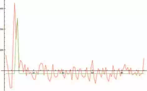
Fig. 14. Analytic programming experimental result. Red colour represents original data from test set (Fig. 9), while green colour represents modelling data using formula (6)
Conclusion
In this chapter, a short introduction into the field of pattern recognition using system adaptation, which is represented via time series, has been given. Two possible approaches were used from the framework of softcomputing methods. The first approach was based on analytic programming and the second one was based on artificial neural networks. Both types of used neural networks (e.g. Hebb and backpropagation networks) as well as analytic programming demonstrated ability to manage to learn and recognize given patterns in time series, which represents our system behaviour. Our experimental results suggest that for the given class of tasks can be acceptable simple classifiers (we tested the simplest type of Hebb learning). The advantage of simple neural networks is very easy implementation and quick adaptation. Easy implementation allows to realize them at low-performance computers (PLC) and their fast adaptation facilitates the process of testing and finding the appropriate type of network for the given application.
The method of analytic programming described here is universal (from point of view of used evolutionary algorithm), relatively simple, easy to implement and easy to use. Analytic programming can be regarded as an equivalent of genetic programming in program synthesis and new universal method, which can be used by arbitrary evolutionary algorithm. AP is also independent of computer platform (PC, Apple, …) and operation system (Windows, Linux, Mac OS,…) because analytic programming can be realized for example in the Mathematica® environment or in other computer languages. It allows manipulation with symbolic terms and final programs are synthesised by AP of mapping, therefore main benefit of analytic programming is the fact that symbolic regression can be done by arbitrary evolutionary algorithm, as was proofed by comparative study.
According to the results of experimental studies, it can be stated that pattern recognition in our system behaviour using all presented methods was successful. It is not possible to say with certainty, which of them reaches the better results, whether neural networks or analytic programming. Both approaches have an important role in the tasks of pattern recognition.
In the future, we would like to apply pattern recognition tasks with the followed system adaptation methods in SIMATIC environment. SIMATIC (SIMATIC, 2010) is an appropriate application environment for industrial control and automation. SIMATIC platform can be applied at the operational, management and the lowest, physical level. At an operational level, it particularly works as a control of the running processes and monitoring of the production. On the management and physical level it can be used to receive any production instructions from the MES system (Manufacturing Execution System – the corporate ERP system set between customers’ orders and manufacturing systems, lines and robots). At the physical level it is mainly used as links among various sensors and actuators, which are physically involved in the production process (Janošek, 2010). The core consists of the SIMATIC programmable logic computers with sensors and actuators. This system collects information about its surroundings through sensors. Data from the sensors can be provided (e.g. via Ethernet) to proposed and created software tools for pattern recognition in real time, which runs on a powerful computer.